Open and Plot Vector Layers
Last updated on 2025-07-02 | Edit this page
Estimated time: 30 minutes
Overview
Questions
- How can I read, examine and visualize point, line and polygon vector data in R?
Objectives
After completing this episode, participants should be able to…
- Differentiate between point, line, and polygon vector data.
- Load vector data into R.
- Access the attributes of a vector object in R.
Make sure that the sf package and its dependencies are
installed before the workshop. The installation can be lengthy, so
allocate enough extra time before the workshop for solving installation
problems. We recommend one or two installation ‘walk-in’ hours on a day
before the workshop. Also, 15-30 minutes at the beginning of the first
workshop day should be enough to tackle last-minute installation
issues.
Prerequisite
In this lesson you will work with the sf package. Note
that the sf package has some external dependencies, namely
GEOS, PROJ.4, GDAL and UDUNITS, which need to be installed beforehand.
Before starting the lesson, follow the workshop setup instructions for the installation of
sf and its dependencies.
First we need to load the packages we will use in this lesson. We
will use the tidyverse package with which you are already
familiar from the previous lesson. In addition, we need to load the sf package for
working with spatial vector data.
R
library(tidyverse) # wrangle, reshape and visualize data
library(sf) # work with spatial vector data
The ‘sf’ package
sf stands for Simple Features which is a standard
defined by the Open Geospatial Consortium for storing and accessing
geospatial vector data. Read more about simple features and its
implementation in R here.
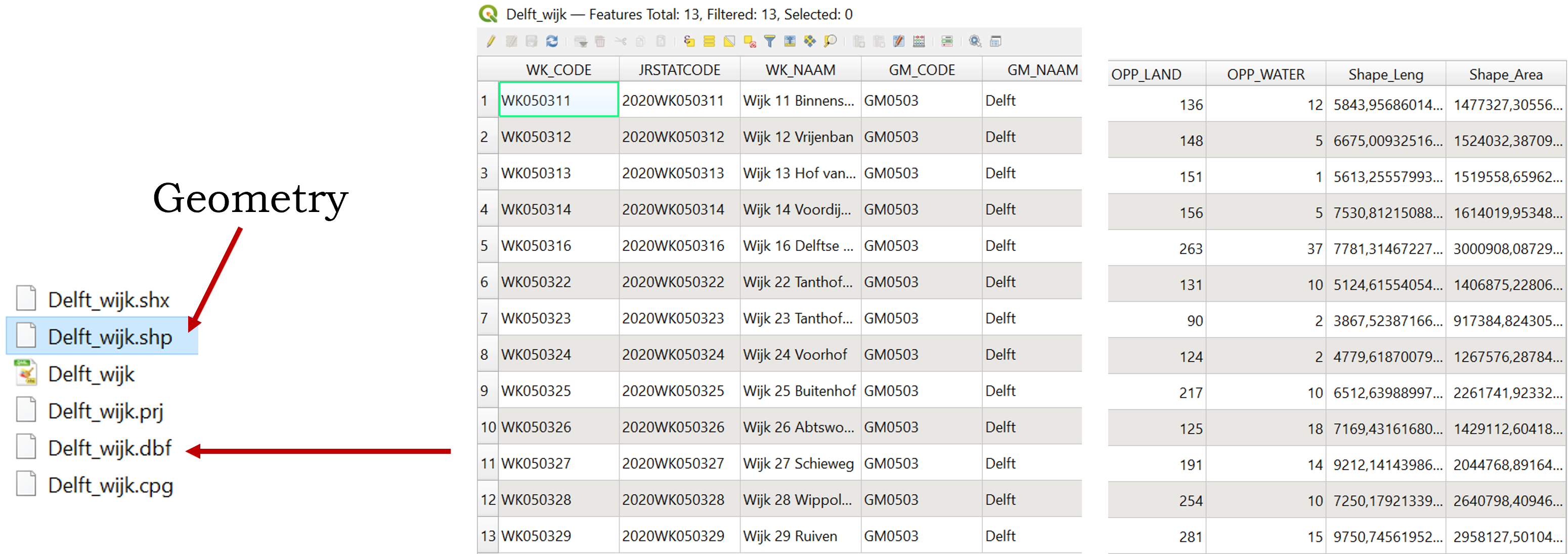
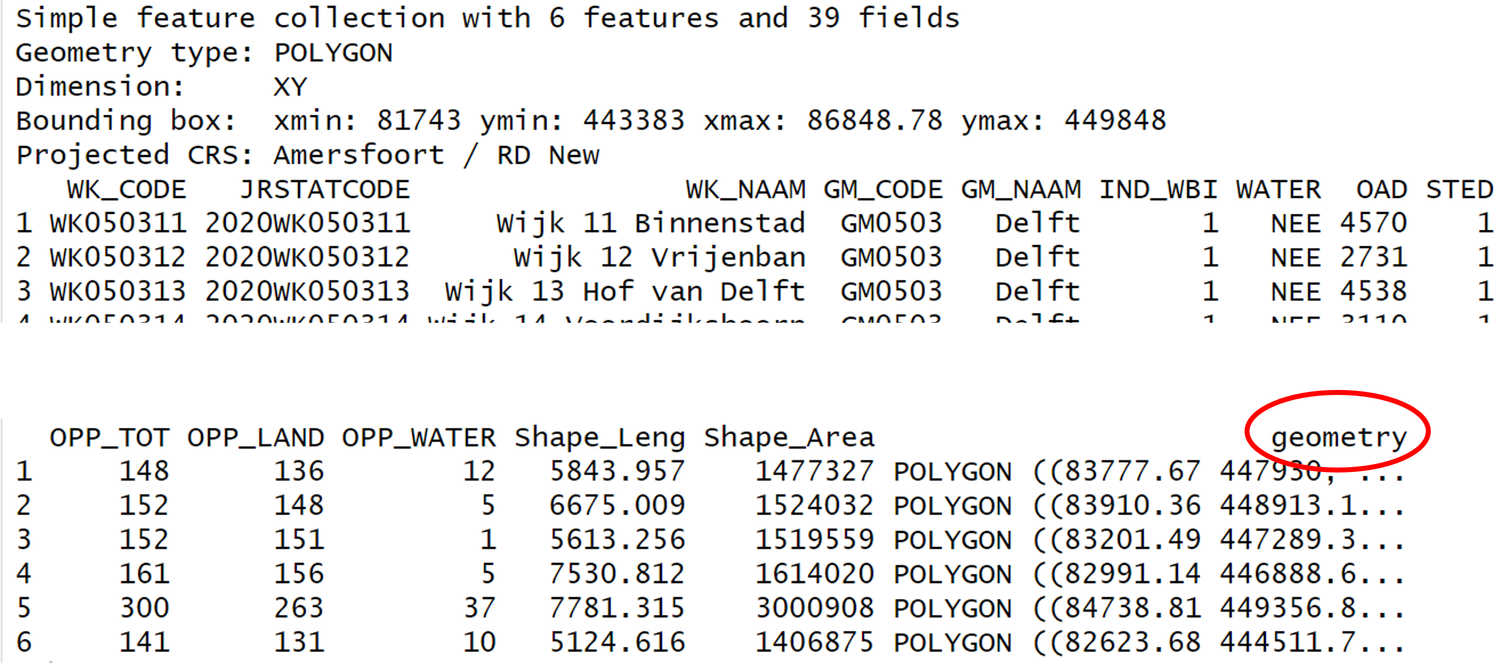
Geometry in QGIS and in R
You may be familiar with GIS software using graphical interfaces like
QGIS. In QGIS, you do not see the geometry in the Attribute Table but it
is directly displayed in the map view. In R, however, the geometry is
stored in a column called geometry.
Import shapefiles
Let’s start by opening a shapefile. Shapefiles are a common file
format to store spatial vector data used in GIS software. Note that a
shapefile consists of multiple files and it is important to keep them
all together in the same location. We will read a shapefile with the
administrative boundary of Delft with the function
st_read() from the sf package.
R
boundary_Delft <- st_read("data/delft-boundary.shp", quiet = TRUE)
All ‘sf’ functions start with ‘st_’
Note that all functions from the sf package start with
the standard prefix st_ which stands for Spatial Type. This
is helpful in at least two ways:
- it allows for easy autocompletion of function names in RStudio, and
- it makes the interaction with or translation to/from software using the simple features standard like PostGIS easy.
Shapefiles vs. GeoPackage
Shapefiles are increasingly being replaced by more modern formats like GeoPackage. An advantage of GeoPackage is that it is a single file that can store multiple layers and attributes, whereas shapefiles consist of multiple files. However, shapefiles are still widely used and are a good starting point for learning about spatial data.
Spatial Metadata
By default (with quiet = FALSE), the
st_read() function provides a message with a summary of
metadata about the file that was read in.
R
st_read("data/delft-boundary.shp")
OUTPUT
Reading layer `delft-boundary' from data source
  `/home/runner/work/r-geospatial-urban/r-geospatial-urban/site/built/data/delft-boundary.shp'
  using driver `ESRI Shapefile'
Simple feature collection with 1 feature and 1 field
Geometry type: POLYGON
Dimension:     XY
Bounding box:  xmin: 4.320218 ymin: 51.96632 xmax: 4.407911 ymax: 52.0326
Geodetic CRS:  WGS 84
To examine the metadata in more detail, we can use other, more
specialised, functions from the sf package. The
st_geometry_type() function, for instance, gives us
information about the geometry type, which in this case is
POLYGON.
R
st_geometry_type(boundary_Delft)
OUTPUT
[1] POLYGON
18 Levels: GEOMETRY POINT LINESTRING POLYGON MULTIPOINT ... TRIANGLE
Geometry types
The sf package supports the following common geometry
types: POINT, LINESTRING,
POLYGON, MULTIPOINT,
MULTILINESTRING, MULTIPOLYGON,
GEOMETRYCOLLECTION. More information about support for
these and other geometry types can be found in the sf package
documentation.
The st_crs() function returns the coordinate reference
system (CRS) used by the shapefile, which in this case is
WGS 84 and has the unique reference code
EPSG: 4326.
R
st_crs(boundary_Delft)
OUTPUT
Coordinate Reference System:
  User input: WGS 84
  wkt:
GEOGCRS["WGS 84",
    DATUM["World Geodetic System 1984",
        ELLIPSOID["WGS 84",6378137,298.257223563,
            LENGTHUNIT["metre",1]]],
    PRIMEM["Greenwich",0,
        ANGLEUNIT["degree",0.0174532925199433]],
    CS[ellipsoidal,2],
        AXIS["latitude",north,
            ORDER[1],
            ANGLEUNIT["degree",0.0174532925199433]],
        AXIS["longitude",east,
            ORDER[2],
            ANGLEUNIT["degree",0.0174532925199433]],
    ID["EPSG",4326]]
Examining the output of ‘st_crs()’
As the output of st_crs() can be long, you can use
$Name and $epsg after the crs()
call to extract the projection name and EPSG code respectively.
R
st_crs(boundary_Delft)$Name
OUTPUT
[1] "WGS 84"R
st_crs(boundary_Delft)$epsg
OUTPUT
[1] 4326The $ operator is used to extract a specific part of an
object. We used it in a previous
episode to subset a data frame by column name. In this case, it is
used to extract named elements stored in a crs object. For
more information, see the
documentation of the st_crs function.
The st_bbox() function shows the extent of the
layer.
R
st_bbox(boundary_Delft)
OUTPUT
     xmin      ymin      xmax      ymax
 4.320218 51.966316  4.407911 52.032599
As WGS 84 is a geographic CRS, the
extent of the shapefile is displayed in degrees. We need a
projected CRS, which in the case of the Netherlands is
the Amersfoort / RD New projection. To reproject our
shapefile, we will use the st_transform() function. For the
crs argument we can use the EPSG code of the CRS we want to
use, which is 28992 for the Amersfort / RD New
projection. To check the EPSG code of any CRS, we can check this
website: https://epsg.io/
R
boundary_Delft <- st_transform(boundary_Delft, crs = 28992)
st_crs(boundary_Delft)$Name
OUTPUT
[1] "Amersfoort / RD New"R
st_crs(boundary_Delft)$epsg
OUTPUT
[1] 28992Notice that the bounding box is measured in meters after the
transformation. The $units_gdal named element confirms that
the new CRS uses metric units.
R
st_bbox(boundary_Delft)
OUTPUT
     xmin      ymin      xmax      ymax
 81743.00 442446.21  87703.78 449847.95
R
st_crs(boundary_Delft)$units_gdal
OUTPUT
[1] "metre"We confirm the transformation by examining the reprojected shapefile.
R
boundary_Delft
OUTPUT
Simple feature collection with 1 feature and 1 field
Geometry type: POLYGON
Dimension:     XY
Bounding box:  xmin: 81743 ymin: 442446.2 xmax: 87703.78 ymax: 449848
Projected CRS: Amersfoort / RD New
  osm_id                       geometry
1 324269 POLYGON ((87703.78 442651, ...
More about CRS
Read more about Coordinate Reference Systems in the previous episode. We will also practice transformation between CRS in Handling Spatial Projection & CRS.
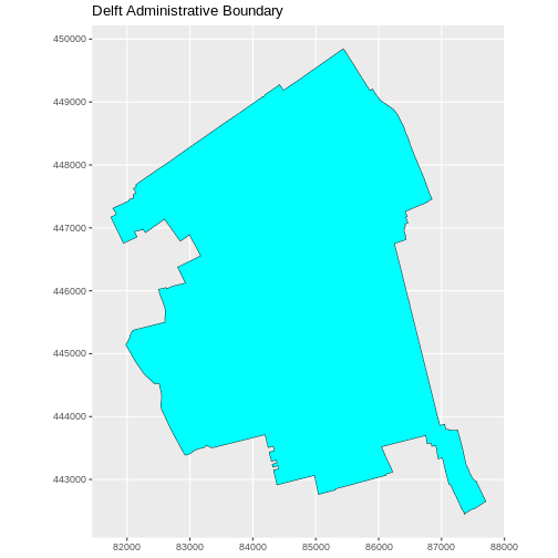
Plot a vector layer
Now, let’s plot this shapefile. You are already familiar with the
ggplot2 package from Introduction to Visualisation.
ggplot2 has special geom_ functions for
spatial data. We will use the geom_sf() function for
sf data. We use coord_sf() to ensure that the
coordinates shown on the two axes are displayed in meters.
R
ggplot(data = boundary_Delft) +
  geom_sf(size = 3, color = "black", fill = "cyan1") +
  labs(title = "Delft Administrative Boundary") +
  coord_sf(datum = st_crs(28992)) # displays the axes in meters
Challenge: Import line and point vector layers
Read in delft-streets.shp and
delft-leisure.shp and assign them to
lines_Delft and points_Delft respectively.
Answer the following questions:
- What is the CRS and extent for each object?
- Do the files contain points, lines, or polygons?
- How many features are in each file?
R
lines_Delft <- st_read("data/delft-streets.shp")
points_Delft <- st_read("data/delft-leisure.shp")
We can check the type of type of geometry with the
st_geometry_type() function. lines_Delft
contains "LINESTRING" geometry and
points_Delft is made of "POINT"
geometries.
R
st_geometry_type(lines_Delft)[1]
OUTPUT
[1] LINESTRING
18 Levels: GEOMETRY POINT LINESTRING POLYGON MULTIPOINT ... TRIANGLE
R
st_geometry_type(points_Delft)[2]
OUTPUT
[1] POINT
18 Levels: GEOMETRY POINT LINESTRING POLYGON MULTIPOINT ... TRIANGLE
Both lines_Delft and points_Delft are in
EPSG:28992.
R
st_crs(lines_Delft)$epsg
OUTPUT
[1] 28992R
st_crs(points_Delft)$epsg
OUTPUT
[1] 28992When looking at the bounding boxes with the st_bbox()
function, we see the spatial extent of the two objects in a projected
CRS using meters as units. lines_Delft() and
points_Delft have similar extents.
R
st_bbox(lines_Delft)
OUTPUT
     xmin      ymin      xmax      ymax
 81759.58 441223.13  89081.41 449845.81
R
st_bbox(points_Delft)
OUTPUT
     xmin      ymin      xmax      ymax
 81863.21 442621.15  87370.15 449345.08
Key Points
- Metadata for vector layers include geometry type, CRS, and extent
and can be examined with the
sffunctionsst_geometry_type(),st_crs(), andst_bbox(), respectively. - Load spatial objects into R with the
sffunctionst_read(). - Spatial objects can be plotted directly with
ggplot2using thegeom_sf()function. No need to convert to a data frame.