Intro to Raster Data
Last updated on 2025-07-02 | Edit this page
Overview
Questions
- What is a raster dataset?
- How do I import, examine and plot raster data in R?
Objectives
After completing this episode, participants should be able to…
- Import rasters into R using the
terrapackage. - Explore raster attributes and metadata using the
terrapackage. - Plot a raster file in R using the
ggplot2package. - Describe the difference between single- and multi-band rasters.
Things you’ll need to complete this episode
See the setup instructions for detailed information about the software, data, and other prerequisites you will need to work through the examples in this episode.
This lesson uses the terra package in particular. If you
have not installed it yet, do so by running
install.packages("terra") before loading it with
library(terra).
In this lesson, we will work with raster data. We will start with an introduction of the fundamental principles and metadata needed to work with raster data in R. We will discuss some of the core metadata elements needed to understand raster data in R, including CRS and resolution.
We continue to work with the tidyverse package and we
will use the terra package to work with raster data. Make
sure that you have those packages loaded.
R
library(tidyverse)
library(terra)
The data used in this lesson
In this and lesson, we will use:
- data extracted from the AHN digital elevation dataset of the Netherlands for the TU Delft campus area; and
- high-resolution RGB aerial photos of the TU Delft library obtained from Beeldmateriaal Nederland.
View Raster File Attributes
We will be working with a series of GeoTIFF files in this lesson. The
GeoTIFF format contains a set of embedded tags with metadata about the
raster data. We can use the function describe() from the
terra package to get information about our raster. It is
recommended to do this before importing the data. We first examine the
file tud-dsm-5m.tif.
R
describe("data/tud-dsm-5m.tif")
OUTPUT
 [1] "Driver: GTiff/GeoTIFF"
 [2] "Files: data/tud-dsm-5m.tif"
 [3] "Size is 722, 386"
 [4] "Coordinate System is:"
 [5] "PROJCRS[\"Amersfoort / RD New\","
 [6] "    BASEGEOGCRS[\"Amersfoort\","
 [7] "        DATUM[\"Amersfoort\","
 [8] "            ELLIPSOID[\"Bessel 1841\",6377397.155,299.1528128,"
 [9] "                LENGTHUNIT[\"metre\",1]]],"
[10] "        PRIMEM[\"Greenwich\",0,"
[11] "            ANGLEUNIT[\"degree\",0.0174532925199433]],"
[12] "        ID[\"EPSG\",4289]],"
[13] "    CONVERSION[\"RD New\","
[14] "        METHOD[\"Oblique Stereographic\","
[15] "            ID[\"EPSG\",9809]],"
[16] "        PARAMETER[\"Latitude of natural origin\",52.1561605555556,"
[17] "            ANGLEUNIT[\"degree\",0.0174532925199433],"
[18] "            ID[\"EPSG\",8801]],"
[19] "        PARAMETER[\"Longitude of natural origin\",5.38763888888889,"
[20] "            ANGLEUNIT[\"degree\",0.0174532925199433],"
[21] "            ID[\"EPSG\",8802]],"
[22] "        PARAMETER[\"Scale factor at natural origin\",0.9999079,"
[23] "            SCALEUNIT[\"unity\",1],"
[24] "            ID[\"EPSG\",8805]],"
[25] "        PARAMETER[\"False easting\",155000,"
[26] "            LENGTHUNIT[\"metre\",1],"
[27] "            ID[\"EPSG\",8806]],"
[28] "        PARAMETER[\"False northing\",463000,"
[29] "            LENGTHUNIT[\"metre\",1],"
[30] "            ID[\"EPSG\",8807]]],"
[31] "    CS[Cartesian,2],"
[32] "        AXIS[\"easting (X)\",east,"
[33] "            ORDER[1],"
[34] "            LENGTHUNIT[\"metre\",1]],"
[35] "        AXIS[\"northing (Y)\",north,"
[36] "            ORDER[2],"
[37] "            LENGTHUNIT[\"metre\",1]],"
[38] "    USAGE["
[39] "        SCOPE[\"Engineering survey, topographic mapping.\"],"
[40] "        AREA[\"Netherlands - onshore, including Waddenzee, Dutch Wadden Islands and 12-mile offshore coastal zone.\"],"
[41] "        BBOX[50.75,3.2,53.7,7.22]],"
[42] "    ID[\"EPSG\",28992]]"
[43] "Data axis to CRS axis mapping: 1,2"
[44] "Origin = (83565.000000000000000,447180.000000000000000)"
[45] "Pixel Size = (5.000000000000000,-5.000000000000000)"
[46] "Metadata:"
[47] "  AREA_OR_POINT=Area"
[48] "Image Structure Metadata:"
[49] "  INTERLEAVE=BAND"
[50] "Corner Coordinates:"
[51] "Upper Left  (   83565.000,  447180.000) (  4d20'49.32\"E, 52d 0'33.67\"N)"
[52] "Lower Left  (   83565.000,  445250.000) (  4d20'50.77\"E, 51d59'31.22\"N)"
[53] "Upper Right (   87175.000,  447180.000) (  4d23'58.60\"E, 52d 0'35.30\"N)"
[54] "Lower Right (   87175.000,  445250.000) (  4d23'59.98\"E, 51d59'32.85\"N)"
[55] "Center      (   85370.000,  446215.000) (  4d22'24.67\"E, 52d 0' 3.27\"N)"
[56] "Band 1 Block=722x2 Type=Float32, ColorInterp=Gray"
We will be using this information throughout this episode. By the end of the episode, you will be able to explain and understand the output above.
Open a Raster in R
Now that we’ve previewed the metadata for our GeoTIFF, let’s import
this raster file into R and explore its metadata more closely. We can
use the rast() function to import a raster file in R.
Data tip - Object names
To improve code readability, use file and object names that make it
clear what is in the file. The raster data for this episode contain the
TU Delft campus and its surroundings so we will use the naming
convention <DATATYPE>_TUD. The first object is a
Digital Surface Model (DSM) in GeoTIFF format stored in a file
tud-dsm-5m.tif which we will load into an object named
according to our naming convention DSM_TUD.
Let’s load our raster file into R and view its data structure.
R
DSM_TUD <- rast("data/tud-dsm-5m.tif")
DSM_TUD
OUTPUT
class       : SpatRaster
size        : 386, 722, 1  (nrow, ncol, nlyr)
resolution  : 5, 5  (x, y)
extent      : 83565, 87175, 445250, 447180  (xmin, xmax, ymin, ymax)
coord. ref. : Amersfoort / RD New (EPSG:28992)
source      : tud-dsm-5m.tif
name        : tud-dsm-5m
The information above includes a report on dimension, resolution,
extent and CRS, but no information about the values. Similar to other
data structures in R like vectors and data frames, descriptive
statistics for raster data can be retrieved with the
summary() function.
R
summary(DSM_TUD)
WARNING
Warning: [summary] used a sampleOUTPUT
   tud.dsm.5m
 Min.   :-5.2235
 1st Qu.:-0.7007
 Median : 0.5462
 Mean   : 2.5850
 3rd Qu.: 4.4596
 Max.   :89.7838
This output gives us information about the range of values in the
DSM. We can see, for instance, that the lowest elevation is
-5.2235, the highest is 89.7838. But note the
warning. Unless you force R to calculate these statistics using every
cell in the raster, it will take a random sample of 100,000 cells and
calculate from them instead. To force calculation all the values, you
can use the function values:
R
summary(values(DSM_TUD))
OUTPUT
   tud-dsm-5m
 Min.   :-5.3907
 1st Qu.:-0.7008
 Median : 0.5573
 Mean   : 2.5886
 3rd Qu.: 4.4648
 Max.   :92.0810
With a summary on all cells of the raster, the values range from a
smaller minimum of -5.3907 to a higher maximum of
92.0910.
To visualise the DSM in R using ggplot2, we need to
convert it to a data frame. We learned about data frames in an earlier lesson. The terra
package has the built-in method as.data.frame() for
conversion to a data frame.
R
DSM_TUD_df <- as.data.frame(DSM_TUD, xy = TRUE)
Now when we view the structure of our data, we will see a standard
data frame format in which every row is a cell from the raster, each
containing information about the x and y
coordinates and the raster value stored in the tud-dsm-5m
column.
R
str(DSM_TUD_df)
OUTPUT
'data.frame':	278692 obs. of  3 variables:
 $ x         : num  83568 83572 83578 83582 83588 ...
 $ y         : num  447178 447178 447178 447178 447178 ...
 $ tud-dsm-5m: num  10.34 8.64 1.25 1.12 2.13 ...
We can use ggplot() to plot this data with a specific
geom_ function called geom_raster(). We will
make the colour scale in our plot colour-blindness friendly with
scale_fill_viridis_c, introduced in an earlier lesson. We will also
use the coord_equal() function to ensure that the units
(meters in our case) on the two axes are equal.
R
ggplot() +
  geom_raster(data = DSM_TUD_df, aes(x = x, y = y, fill = `tud-dsm-5m`)) +
  scale_fill_viridis_c(option = "turbo") +
  coord_equal()
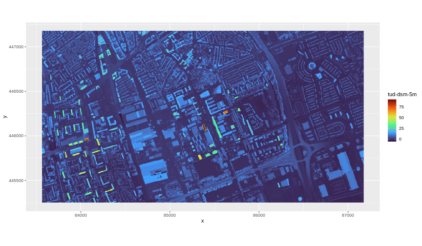
ggplot2 using the viridis color scale
Plotting tip
The "turbo" scale in our code provides a good
contrasting scale for our raster, but another colour scale may be
preferred when plotting other rasters. More information about the
viridis palette used above can be found in the viridis
package documentation.
Plotting tip
For faster previews, you can use the plot() function on
a terra object.
View Raster Coordinate Reference System (CRS)
The map above shows our Digital Surface Model (DSM), that is, the elevation of our study site including buildings and vegetation. From the legend we can confirm that the maximum elevation is around 90, but we cannot tell whether that is 90 feet or 90 meters because the legend does not show us the units. We can look at the metadata of our object to see what the units are. Much of the metadata that we are interested in is part of the CRS.
Now we will see how features of the CRS appear in our data file and what meaning they have.
We can view the CRS string associated with our R object using the
crs() function.
R
crs(DSM_TUD, proj = TRUE)
OUTPUT
[1] "+proj=sterea +lat_0=52.1561605555556 +lon_0=5.38763888888889 +k=0.9999079 +x_0=155000 +y_0=463000 +ellps=bessel +units=m +no_defs"Challenge: What units are our data in?
+units=m in the output of the code above tells us that
our data is in meters (m).
Understanding CRS in PROJ.4 format
The CRS for our data is given to us by R in PROJ.4 format. Let’s
break down the pieces of a PROJ.4 string. The string contains all of the
individual CRS elements that R or another GIS might need. Each element
is specified with a + sign, similar to how a
.csv file is delimited or broken up by a ,.
After each + we see the CRS element such as projection
(proj=) being defined.
See more about CRS and PROJ.4 strings in this lesson.
Calculate Raster Min and Max values
It is useful to know the minimum and maximum values of a raster dataset. In this case, as we are working with elevation data, these values represent the minimum-to-maximum elevation range at our site.
Raster statistics are often calculated and embedded in a GeoTIFF for us. We can view these values:
R
minmax(DSM_TUD)
OUTPUT
    tud-dsm-5m
min        Inf
max       -Inf
Data tip - Set min and max values
If the min and max values are
Inf and -Inf respectively, it means that they
haven’t been calculated. We can calculate them using the
setMinMax() function.
R
DSM_TUD <- setMinMax(DSM_TUD)
A call to minmax(DSM_TUD) will now give us the correct
values. Alternatively, min(values()) and
max(values()) will return the minimum and maximum values
respectively.
R
min(values(DSM_TUD))
OUTPUT
[1] -5.39069R
max(values(DSM_TUD))
OUTPUT
[1] 92.08102We can see that the elevation at our site ranges from
-5.39069m to 92.08102m.
Raster bands
The Digital Surface Model object (DSM_TUD) that we have
been working with is a single band raster. This means that there is only
one layer stored in the raster: surface elevation in meters for one time
period.
We can view the number of bands in a raster using the
nlyr() function.
R
nlyr(DSM_TUD)
OUTPUT
[1] 1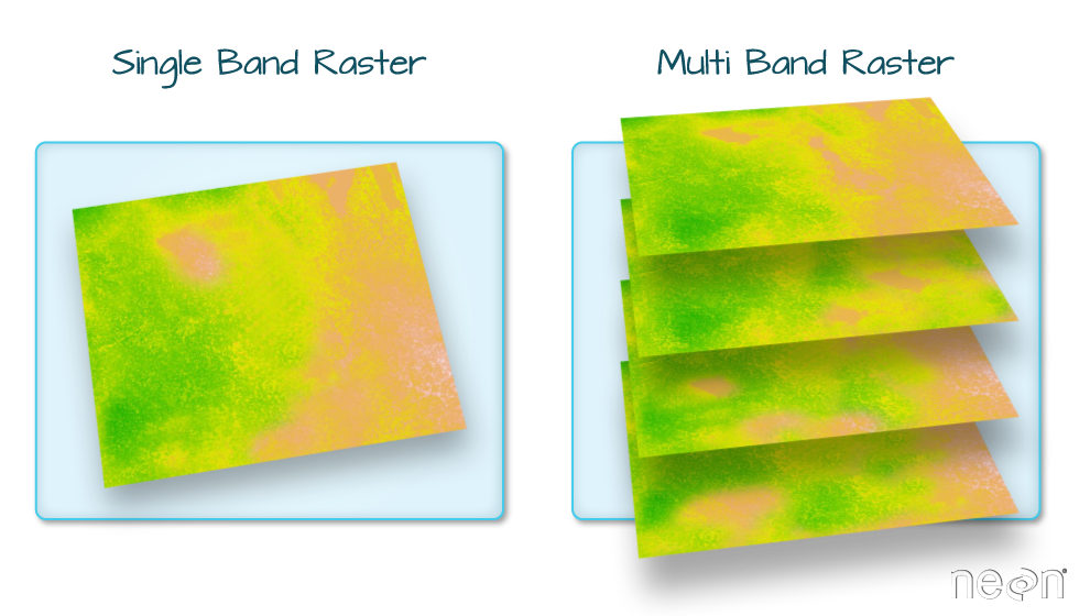
Our DSM data has only one band. However, raster data can also be multi-band, meaning that one raster file contains data for more than one variable or time period for each cell. We will discuss multi-band raster data in a later episode.
Creating a histogram of raster values
A histogram can be used to inspect the distribution of raster values
visually. It can show if there are values above the maximum or below the
minimum of the expected range. We can plot a histogram using the
ggplot2 function geom_histogram(). Histograms
are often useful in identifying outliers and bad data values in our
raster data. Read more on the use of histograms in this
lesson
Challenge: Explore raster metadata
Use describe() to determine the following about the
tud-dsm-hill.tif file:
- Does this file have the same CRS as
DSM_TUD? - What is the resolution of the raster data?
- How large would a 5x5 pixel area be on the Earth’s surface?
- Is the file a multi- or single-band raster?
Note that this file is a hillshade raster. We will learn about hillshades in the Working with Multi-band Rasters in R episode.
R
describe("data/tud-dsm-5m-hill.tif")
OUTPUT
 [1] "Driver: GTiff/GeoTIFF"
 [2] "Files: data/tud-dsm-5m-hill.tif"
 [3] "Size is 722, 386"
 [4] "Coordinate System is:"
 [5] "PROJCRS[\"Amersfoort / RD New\","
 [6] "    BASEGEOGCRS[\"Amersfoort\","
 [7] "        DATUM[\"Amersfoort\","
 [8] "            ELLIPSOID[\"Bessel 1841\",6377397.155,299.1528128,"
 [9] "                LENGTHUNIT[\"metre\",1]]],"
[10] "        PRIMEM[\"Greenwich\",0,"
[11] "            ANGLEUNIT[\"degree\",0.0174532925199433]],"
[12] "        ID[\"EPSG\",4289]],"
[13] "    CONVERSION[\"RD New\","
[14] "        METHOD[\"Oblique Stereographic\","
[15] "            ID[\"EPSG\",9809]],"
[16] "        PARAMETER[\"Latitude of natural origin\",52.1561605555556,"
[17] "            ANGLEUNIT[\"degree\",0.0174532925199433],"
[18] "            ID[\"EPSG\",8801]],"
[19] "        PARAMETER[\"Longitude of natural origin\",5.38763888888889,"
[20] "            ANGLEUNIT[\"degree\",0.0174532925199433],"
[21] "            ID[\"EPSG\",8802]],"
[22] "        PARAMETER[\"Scale factor at natural origin\",0.9999079,"
[23] "            SCALEUNIT[\"unity\",1],"
[24] "            ID[\"EPSG\",8805]],"
[25] "        PARAMETER[\"False easting\",155000,"
[26] "            LENGTHUNIT[\"metre\",1],"
[27] "            ID[\"EPSG\",8806]],"
[28] "        PARAMETER[\"False northing\",463000,"
[29] "            LENGTHUNIT[\"metre\",1],"
[30] "            ID[\"EPSG\",8807]]],"
[31] "    CS[Cartesian,2],"
[32] "        AXIS[\"easting (X)\",east,"
[33] "            ORDER[1],"
[34] "            LENGTHUNIT[\"metre\",1]],"
[35] "        AXIS[\"northing (Y)\",north,"
[36] "            ORDER[2],"
[37] "            LENGTHUNIT[\"metre\",1]],"
[38] "    USAGE["
[39] "        SCOPE[\"Engineering survey, topographic mapping.\"],"
[40] "        AREA[\"Netherlands - onshore, including Waddenzee, Dutch Wadden Islands and 12-mile offshore coastal zone.\"],"
[41] "        BBOX[50.75,3.2,53.7,7.22]],"
[42] "    ID[\"EPSG\",28992]]"
[43] "Data axis to CRS axis mapping: 1,2"
[44] "Origin = (83565.000000000000000,447180.000000000000000)"
[45] "Pixel Size = (5.000000000000000,-5.000000000000000)"
[46] "Metadata:"
[47] "  AREA_OR_POINT=Area"
[48] "Image Structure Metadata:"
[49] "  INTERLEAVE=BAND"
[50] "Corner Coordinates:"
[51] "Upper Left  (   83565.000,  447180.000) (  4d20'49.32\"E, 52d 0'33.67\"N)"
[52] "Lower Left  (   83565.000,  445250.000) (  4d20'50.77\"E, 51d59'31.22\"N)"
[53] "Upper Right (   87175.000,  447180.000) (  4d23'58.60\"E, 52d 0'35.30\"N)"
[54] "Lower Right (   87175.000,  445250.000) (  4d23'59.98\"E, 51d59'32.85\"N)"
[55] "Center      (   85370.000,  446215.000) (  4d22'24.67\"E, 52d 0' 3.27\"N)"
[56] "Band 1 Block=722x11 Type=Byte, ColorInterp=Gray"
[57] "  NoData Value=0"
More resources
- See the manual and tutorials of the
terrapackage on https://rspatial.org/.
Key Points
- The GeoTIFF file format includes metadata about the raster data that
can be inspected with the
describe()function from theterrapackage. - To plot raster data with the
ggplot2package, we need to convert them to data frames. - PROJ is a widely used standard format to store, represent and transform CRS.
- Histograms are useful to identify missing or bad data values.