Explore and plot by vector layer attributes
Last updated on 2025-07-02 | Edit this page
Overview
Questions
- How can I examine the attributes of a vector layer?
Objectives
After completing this episode, participants should be able to…
Query attributes of a vector object.
Subset vector objects using specific attribute values.
Plot a vector feature, coloured by unique attribute values.
Query Vector Feature Metadata
Let’s have a look at the content of the loaded data, starting with
lines_Delft. In essence, an "sf" object is a
data.frame with a “sticky” geometry column and some extra metadata, like
the CRS, extent and geometry type we examined earlier.
R
lines_Delft
OUTPUT
Simple feature collection with 11244 features and 2 fields
Geometry type: LINESTRING
Dimension:     XY
Bounding box:  xmin: 81759.58 ymin: 441223.1 xmax: 89081.41 ymax: 449845.8
Projected CRS: Amersfoort / RD New
First 10 features:
    osm_id  highway                       geometry
1  4239535 cycleway LINESTRING (86399.68 448599...
2  4239536 cycleway LINESTRING (85493.66 448740...
3  4239537 cycleway LINESTRING (85493.66 448740...
4  4239620  footway LINESTRING (86299.01 448536...
5  4239621  footway LINESTRING (86307.35 448738...
6  4239674  footway LINESTRING (86299.01 448536...
7  4310407  service LINESTRING (84049.47 447778...
8  4310808    steps LINESTRING (84588.83 447828...
9  4348553  footway LINESTRING (84527.26 447861...
10 4348575  footway LINESTRING (84500.15 447255...
This means that we can examine and manipulate them as data frames.
For instance, we can look at the number of variables (columns in a data
frame) with ncol().
R
ncol(lines_Delft)
OUTPUT
[1] 3In the case of point_Delft those columns are
"osm_id", "highway" and
"geometry". We can check the names of the columns with the
function names().
R
names(lines_Delft)
OUTPUT
[1] "osm_id" "highway" "geometry"The geometry as a column
Note that in R the geometry is just another column and counts towards
the number returned by ncol(). This is different from GIS
software with graphical user interfaces, where the geometry is displayed
in a viewport not as a column in the attribute table.
We can also preview the content of the object by looking at the first
6 rows with the head() function, which in the case of an
sf object is similar to examining the object directly.
R
head(lines_Delft)
OUTPUT
Simple feature collection with 6 features and 2 fields
Geometry type: LINESTRING
Dimension:     XY
Bounding box:  xmin: 85107.1 ymin: 448400.3 xmax: 86399.68 ymax: 449076.2
Projected CRS: Amersfoort / RD New
   osm_id  highway                       geometry
1 4239535 cycleway LINESTRING (86399.68 448599...
2 4239536 cycleway LINESTRING (85493.66 448740...
3 4239537 cycleway LINESTRING (85493.66 448740...
4 4239620  footway LINESTRING (86299.01 448536...
5 4239621  footway LINESTRING (86307.35 448738...
6 4239674  footway LINESTRING (86299.01 448536...
Explore values within one attribute
Using the $ operator, we can examine the content of a
single field of our lines object. Let’s have a look at the
highway field, a categorical variable stored in the
lines_Delft object as character. To avoid
displaying all 11244 values of highway, we will preview it
with the head() function:
R
head(lines_Delft$highway, 10)
OUTPUT
 [1] "cycleway" "cycleway" "cycleway" "footway"  "footway"  "footway"
 [7] "service"  "steps"    "footway"  "footway"
The first rows returned by the head() function do not
necessarily contain all unique values within the highway
field. To see all unique values, we can use the unique()
function. This function extracts all possible values of a character
variable. For the highway field, this returns all types of
roads stored in lines_Delft.
R
unique(lines_Delft$highway)
OUTPUT
 [1] "cycleway"       "footway"        "service"        "steps"
 [5] "residential"    "unclassified"   "construction"   "secondary"
 [9] "busway"         "living_street"  "motorway_link"  "tertiary"
[13] "track"          "motorway"       "path"           "pedestrian"
[17] "primary"        "bridleway"      "trunk"          "tertiary_link"
[21] "services"       "secondary_link" "trunk_link"     "primary_link"
[25] "platform"       "proposed"       NA
Using factors in sf objects
R is also able to handle categorical variables called factors,
introduced in an earlier episode.
With factors, we can use the levels() function to show
unique values. To examine unique values of the highway
variable this way, we have to first transform it into a factor with the
factor() function:
R
factor(lines_Delft$highway) |> levels()
OUTPUT
 [1] "bridleway"      "busway"         "construction"   "cycleway"
 [5] "footway"        "living_street"  "motorway"       "motorway_link"
 [9] "path"           "pedestrian"     "platform"       "primary"
[13] "primary_link"   "proposed"       "residential"    "secondary"
[17] "secondary_link" "service"        "services"       "steps"
[21] "tertiary"       "tertiary_link"  "track"          "trunk"
[25] "trunk_link"     "unclassified"
Note that this way the values are shown by default in alphabetical
order and NAs are not displayed, whereas using
unique() returns unique values in the order of their
occurrence in the data frame and it also shows NA
values.
Challenge: Attributes for different spatial classes
Explore the attributes associated with the point_Delft
spatial object.
- How many fields does it have?
- What types of leisure points do the points represent? Give three examples.
- Which of the following is NOT a field of the
point_Delftobject?
-
locationB)leisureC)osm_id
- To find the number of fields, we use the
ncol()function:
R
ncol(point_Delft)
OUTPUT
[1] 3- The types of leisure point are in the column named
leisure.
Using the head() function which displays 6 rows by
default, we only see two values and NAs.
R
head(point_Delft)
OUTPUT
Simple feature collection with 6 features and 2 fields
Geometry type: POINT
Dimension:     XY
Bounding box:  xmin: 83839.59 ymin: 443827.4 xmax: 84967.67 ymax: 447475.5
Projected CRS: Amersfoort / RD New
     osm_id      leisure                  geometry
1 472312297 picnic_table POINT (84144.72 443827.4)
2 480470725       marina POINT (84967.67 446120.1)
3 484697679         <NA> POINT (83912.28 447431.8)
4 484697682         <NA> POINT (83895.43 447420.4)
5 484697691         <NA>   POINT (83839.59 447455)
6 484697814         <NA> POINT (83892.53 447475.5)
We can increase the number of rows with the n argument
(e.g., head(n = 10) to show 10 rows) until we see at least
three distinct values in the leisure column. Note that printing an
sf object will also display the first 10 rows.
R
# you might be lucky to see three distinct values
head(point_Delft, 10)
OUTPUT
Simple feature collection with 10 features and 2 fields
Geometry type: POINT
Dimension:     XY
Bounding box:  xmin: 82485.72 ymin: 443827.4 xmax: 85385.25 ymax: 448341.3
Projected CRS: Amersfoort / RD New
       osm_id       leisure                  geometry
1   472312297  picnic_table POINT (84144.72 443827.4)
2   480470725        marina POINT (84967.67 446120.1)
3   484697679          <NA> POINT (83912.28 447431.8)
4   484697682          <NA> POINT (83895.43 447420.4)
5   484697691          <NA>   POINT (83839.59 447455)
6   484697814          <NA> POINT (83892.53 447475.5)
7   549139430        marina POINT (84479.99 446823.5)
8   603300994 sports_centre POINT (82485.72 445237.5)
9   883518959 sports_centre POINT (85385.25 448341.3)
10 1148515039    playground    POINT (84661.3 446818)
We have our answer (sports_centre is the third value),
but in general this is not a good approach as the first rows might still
have many NAs and three distinct values might still not be
present in the first n rows of the data frame. To remove
NAs, we can use the function na.omit() on the
leisure column to remove NAs completely. Note that we use
the $ operator to examine the content of a single
variable.
R
# this is better
na.omit(point_Delft$leisure) |> head()
OUTPUT
[1] "picnic_table"  "marina"        "marina"        "sports_centre"
[5] "sports_centre" "playground"
To show only unique values, we can use the levels()
function on a factor to only see the first occurrence of each distinct
value. Note NAs are dropped in this case and that we get
the first three of the unique alphabetically ordered values.
R
# this is even better
factor(point_Delft$leisure) |>
  levels() |>
  head(n = 3)
OUTPUT
[1] "dance" "dog_park" "escape_game"- To see a list of all fields names and answer the last question, we
can use the
names()function.
R
names(point_Delft)
OUTPUT
[1] "osm_id" "leisure" "geometry"-
locationis not a field of thepoint_Delftobject.
Subset features
We can use the filter() function to select a subset of
features from a spatial object, just like with data frames. Let’s select
only cycleways from our street data.
R
cycleway_Delft <- lines_Delft |>
  filter(highway == "cycleway")
Our subsetting operation reduces the number of features from 11244 to 1397.
R
nrow(lines_Delft)
OUTPUT
[1] 11244R
nrow(cycleway_Delft)
OUTPUT
[1] 1397This can be useful, for instance, to calculate the total length of
cycleways. For that, we first need to calculate the length of each
segment with st_length()
R
cycleway_Delft <- cycleway_Delft |>
  mutate(length = st_length(geometry))

cycleway_Delft |>
  summarise(total_length = sum(length))
OUTPUT
Simple feature collection with 1 feature and 1 field
Geometry type: MULTILINESTRING
Dimension: XY
Bounding box: xmin: 81759.58 ymin: 441227.3 xmax: 87326.76 ymax: 449834.5
Projected CRS: Amersfoort / RD New
total_length geometry
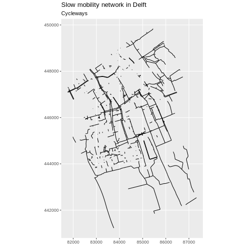
1 115550.1 [m] MULTILINESTRING ((86399.68 ...Now we can plot only the cycleways.
R
ggplot(data = cycleway_Delft) +
  geom_sf() +
  labs(
    title = "Slow mobility network in Delft",
    subtitle = "Cycleways"
  ) +
  coord_sf(datum = st_crs(28992))
Challenge
Challenge: Now with motorways
- Create a new object that only contains the motorways in Delft.
- How many features does the new object have?
- What is the total length of motorways?
- Plot the motorways.
- To create the new object, we first need to see which value of the
highwaycolumn holds motorways. There is a value calledmotorway.
R
unique(lines_Delft$highway)
OUTPUT
 [1] "cycleway"       "footway"        "service"        "steps"
 [5] "residential"    "unclassified"   "construction"   "secondary"
 [9] "busway"         "living_street"  "motorway_link"  "tertiary"
[13] "track"          "motorway"       "path"           "pedestrian"
[17] "primary"        "bridleway"      "trunk"          "tertiary_link"
[21] "services"       "secondary_link" "trunk_link"     "primary_link"
[25] "platform"       "proposed"       NA
We extract only the features with the value
motorway.
R
motorway_Delft <- lines_Delft |>
  filter(highway == "motorway")

motorway_Delft
OUTPUT
Simple feature collection with 48 features and 2 fields
Geometry type: LINESTRING
Dimension:     XY
Bounding box:  xmin: 84501.66 ymin: 442458.2 xmax: 87401.87 ymax: 449205.9
Projected CRS: Amersfoort / RD New
First 10 features:
      osm_id  highway                       geometry
1    7531946 motorway LINESTRING (87395.68 442480...
2    7531976 motorway LINESTRING (87401.87 442467...
3   46212227 motorway LINESTRING (86103.56 446928...
4  120945066 motorway LINESTRING (85724.87 447473...
5  120945068 motorway LINESTRING (85710.31 447466...
6  126548650 motorway LINESTRING (86984.12 443630...
7  126548651 motorway LINESTRING (86714.75 444772...
8  126548653 motorway LINESTRING (86700.23 444769...
9  126548654 motorway LINESTRING (86716.35 444766...
10 126548655 motorway LINESTRING (84961.78 448566...- There are 48 features with the value
motorway.
R
nrow(motorway_Delft)
OUTPUT
[1] 48- The total length of motorways is 14877.4361477941.
R
motorway_Delft_length <- motorway_Delft |>
  mutate(length = st_length(geometry)) |>
  select(everything(), geometry) |>
  summarise(total_length = sum(length))
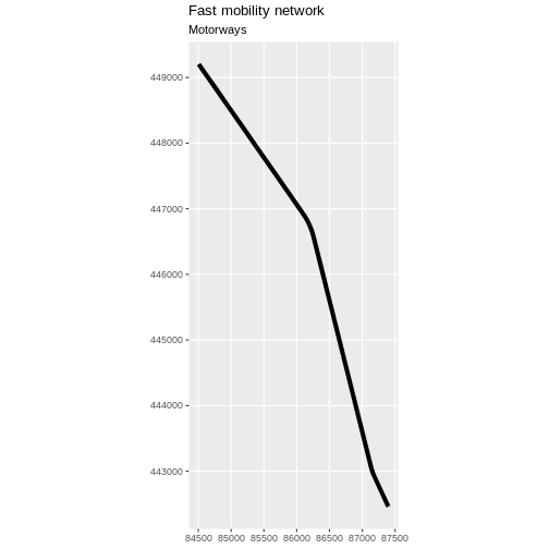
- Plot the motorways.
R
ggplot(data = motorway_Delft) +
  geom_sf(linewidth = 1.5) +
  labs(
    title = "Fast mobility network",
    subtitle = "Motorways"
  ) +
  coord_sf(datum = st_crs(28992))
Customize plots
Let’s say that we want to color different road types with different colors and that we want to determine those colors.
R
unique(lines_Delft$highway)
OUTPUT
 [1] "cycleway"       "footway"        "service"        "steps"
 [5] "residential"    "unclassified"   "construction"   "secondary"
 [9] "busway"         "living_street"  "motorway_link"  "tertiary"
[13] "track"          "motorway"       "path"           "pedestrian"
[17] "primary"        "bridleway"      "trunk"          "tertiary_link"
[21] "services"       "secondary_link" "trunk_link"     "primary_link"
[25] "platform"       "proposed"       NA
If we look at all the unique values of the highway field of our
street network we see more than 20 values. Let’s focus on a subset of
four values to illustrate the use of distinct colours. We filter the
roads that have one of the four given values "motorway",
"primary", "secondary", and
"cycleway". Note that we do this with the %in%
operator which is a more compact equivalent of a series of
== equality conditions joined by the | (or)
operator. We also make sure that the highway column is a factor
column.
R
road_types <- c("motorway", "primary", "secondary", "cycleway")

lines_Delft_selection <- lines_Delft |>
  filter(highway %in% road_types) |>
  mutate(highway = factor(highway, levels = road_types))
Next we define the four colours we want to use, one for each type of
road in our vector object. Note that in R you can use named colours like
"blue", "green", "navy", and
"purple". If you are using RStudio, you will see the named
colours previewed in line. A full list of named colours can be listed
with the colors() function.
R
road_colors <- c("blue", "green", "navy", "purple")
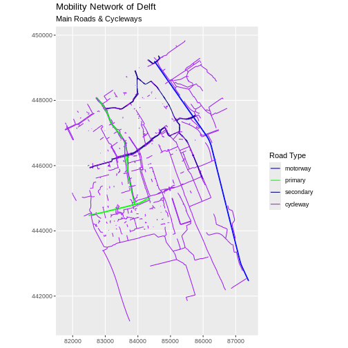
We can use the defined colour palette in a ggplot.
R
ggplot(data = lines_Delft_selection) +
  geom_sf(aes(color = highway)) +
  scale_color_manual(values = road_colors) +
  labs(
    color = "Road Type",
    title = "Mobility Network of Delft",
    subtitle = "Main Roads & Cycleways"
  ) +
  coord_sf(datum = st_crs(28992))
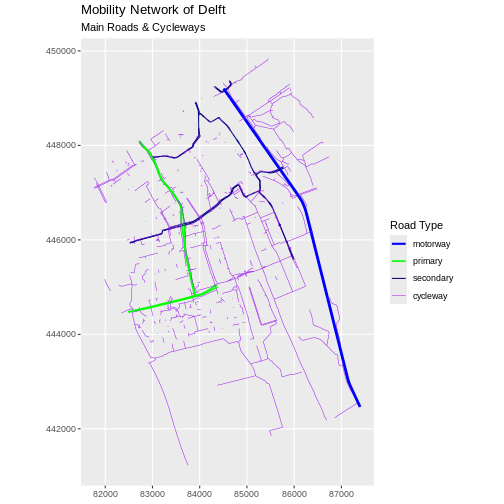
Challenge: Adjust line width
Follow the same steps to add custom line widths for every road type.
Assign the custom values
1,0.75,0.5,0.25in this order to an object calledline_widths. These values will represent line thicknesses that are consistent with the hierarchy of the selected road types.In this case the
linewidthargument, like thecolorargument above, should be within theaes()mapping function and should take the values of the custom line widths.Plot the result, making sure that
linewidthis named the same way ascolorin the legend.
R
line_widths <- c(1, 0.75, 0.5, 0.25)
R
ggplot(data = lines_Delft_selection) +
  geom_sf(aes(color = highway, linewidth = highway)) +
  scale_color_manual(values = road_colors) +
  scale_linewidth_manual(values = line_widths) +
  labs(
    color = "Road Type",
    linewidth = "Road Type",
    title = "Mobility Network of Delft",
    subtitle = "Main Roads & Cycleways"
  ) +
  coord_sf(datum = st_crs(28992))
Challenge: Plot lines by attributes
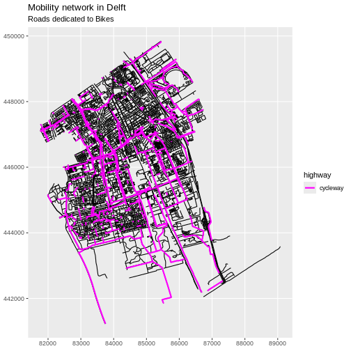
Create a plot that emphasizes only roads where bicycles are allowed. To emphasize this, make the lines where bicycles are not allowed THINNER than the roads where bicycles are allowed. Be sure to add a title and legend to your map. You might consider a color palette that has all bike-friendly roads displayed in a bright color. All other lines can be black.
Tip: geom_sf() can be called multiple times for
multi-layer maps.
R
class(lines_Delft_selection$highway)
OUTPUT
[1] "factor"R
levels(factor(lines_Delft$highway))
OUTPUT
 [1] "bridleway"      "busway"         "construction"   "cycleway"
 [5] "footway"        "living_street"  "motorway"       "motorway_link"
 [9] "path"           "pedestrian"     "platform"       "primary"
[13] "primary_link"   "proposed"       "residential"    "secondary"
[17] "secondary_link" "service"        "services"       "steps"
[21] "tertiary"       "tertiary_link"  "track"          "trunk"
[25] "trunk_link"     "unclassified"
R
# First, create a data frame with only roads where bicycles
# are allowed
lines_Delft_bicycle <- lines_Delft |>
  filter(highway == "cycleway")

# Next, visualise it using ggplot
ggplot(data = lines_Delft) +
  geom_sf() +
  geom_sf(
    data = lines_Delft_bicycle,
    aes(color = highway),
    linewidth = 1
  ) +
  scale_color_manual(values = "magenta") +
  labs(
    title = "Mobility network in Delft",
    subtitle = "Roads dedicated to Bikes"
  ) +
  coord_sf(datum = st_crs(28992))
Key Points
Spatial objects in
sfare similar to standard data frames and can be manipulated using the same functions.Almost any feature of a plot can be customized using the various functions and options in the
ggplot2package.