Reproject Raster Data
Last updated on 2025-07-02 | Edit this page
Overview
Questions
- How do I work with raster data sets that are in different projections?
Objectives
After completing this episode, participants should be able to…
- Reproject a raster in R.
Things you’ll need to complete this episode
See the setup instructions for detailed information about the software, data, and other prerequisites you will need to work through the examples in this episode.
Sometimes we encounter raster datasets that do not “line up” when
plotted or analysed. Rasters that do not line up are most often in
different Coordinate Reference Systems (CRS). This episode explains how
to deal with rasters in different CRS. It will walk through reprojecting
rasters in R using the project() function in the
terra package.
Raster Projection
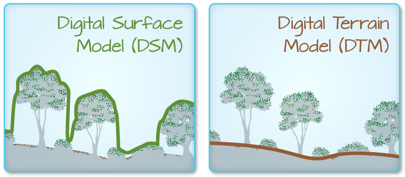
For this episode, we will be working with Digital Terrain Model data. This differs from the surface model data we have been working with so far in that the digital surface model (DSM) includes the tops of trees and buildings, while the digital terrain model (DTM) shows the ground level.
We will be looking at another model (the canopy/building height
model, or CHM) in a later
episode and will see how to calculate the CHM from the DSM and DTM.
Here, we will create a map of the Digital Terrain Model
(DTM_TUD) of TU Delft and its surrounding draped (or
layered) on top of the hillshade (DTM_hill_TUD).
Layering Rasters: Hillshade
We can layer a raster on top of a hillshade raster for the same area, and use a transparency factor to create a 3-dimensional shaded effect. A hillshade is a raster that maps the terrain using light and shadow to create a 3D-looking image that you would see from above when viewing the terrain. We will add a custom colour, making the plot grey.
Read more about layering rasters here.
First, we need to import the DTM and DTM hillshade data.
R
DTM_TUD <- rast("data/tud-dtm-5m.tif")
DTM_hill_TUD <- rast("data/tud-dtm-5m-hill-WGS84.tif")
Next, we will convert each of these datasets to a data frame for
plotting with ggplot.
R
DTM_TUD_df <- as.data.frame(DTM_TUD, xy = TRUE)
DTM_hill_TUD_df <- as.data.frame(DTM_hill_TUD, xy = TRUE)
Now we can create a map of the DTM layered over the hillshade.
R
ggplot() +
  geom_raster(
    data = DTM_TUD_df,
    aes(
      x = x,
      y = y,
      fill = `tud-dtm-5m`
    )
  ) +
  geom_raster(
    data = DTM_hill_TUD_df,
    aes(
      x = x,
      y = y,
      alpha = `tud-dtm-5m-hill`
    )
  ) +
  scale_fill_gradientn(name = "Elevation", colors = terrain.colors(10)) +
  coord_equal()
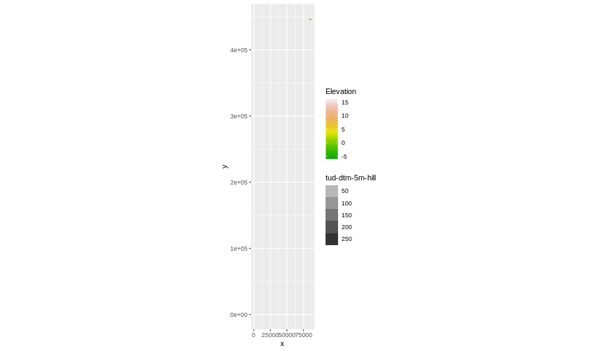 Our results are curious - neither the DTM (
DTM_TUD_df) nor
the hillshade (DTM_hill_TUD_df) are plotted. Let’s try to
plot the DTM on its own to make sure the data are there.
R
ggplot() +
  geom_raster(
    data = DTM_TUD_df,
    aes(
      x = x,
      y = y,
      fill = `tud-dtm-5m`
    )
  ) +
  scale_fill_gradientn(name = "Elevation", colors = terrain.colors(10)) +
  coord_equal()
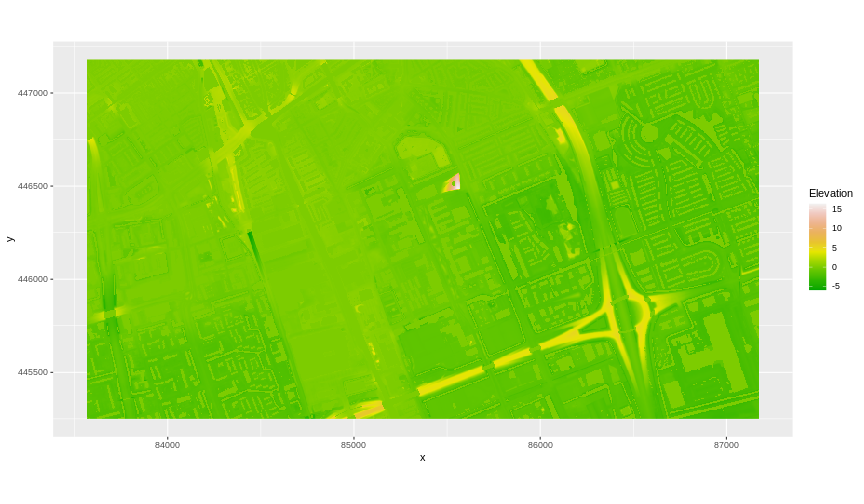
Our DTM seems to contain data and plots just fine.
Next we plot the DTM Hillshade on its own to see whether everything is OK.
R
ggplot() +
  geom_raster(
    data = DTM_hill_TUD_df,
    aes(
      x = x,
      y = y,
      alpha = `tud-dtm-5m-hill`
    )
  ) +
  coord_equal()
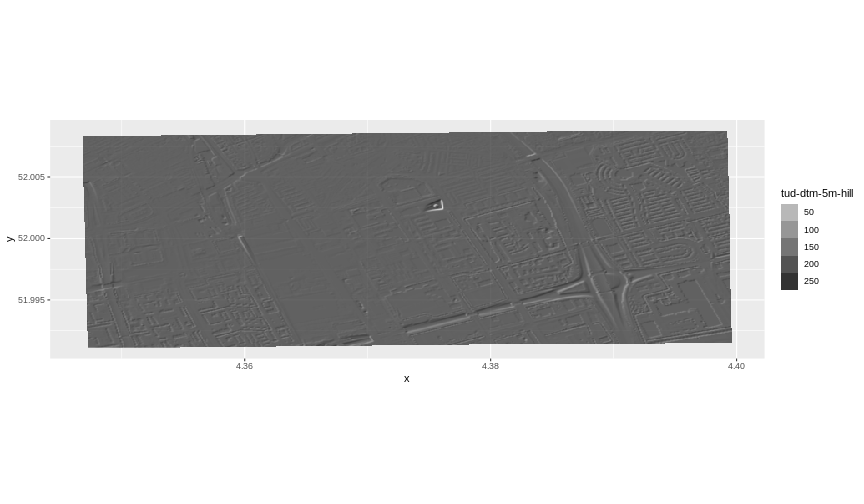
If we examine the axes, we can see that the units (and thus the
projections) of the two rasters differ. In such cases,
ggplot2 will still render the images, but they may not be
visible. The function doesn’t throw an error, but rather completes the
rendering process, which can make it seem like nothing is wrong. To
better understand this, we can compare the Coordinate Reference Systems
(CRSs) of the DTM and hillshade data to see how they differ.
Challenge: compare the CRSs
View the CRS for each of these two datasets. What projection does each use?
R
crs(DTM_TUD, parse = TRUE)
OUTPUT
 [1] "PROJCRS[\"Amersfoort / RD New\","
 [2] "    BASEGEOGCRS[\"Amersfoort\","
 [3] "        DATUM[\"Amersfoort\","
 [4] "            ELLIPSOID[\"Bessel 1841\",6377397.155,299.1528128,"
 [5] "                LENGTHUNIT[\"metre\",1]]],"
 [6] "        PRIMEM[\"Greenwich\",0,"
 [7] "            ANGLEUNIT[\"degree\",0.0174532925199433]],"
 [8] "        ID[\"EPSG\",4289]],"
 [9] "    CONVERSION[\"RD New\","
[10] "        METHOD[\"Oblique Stereographic\","
[11] "            ID[\"EPSG\",9809]],"
[12] "        PARAMETER[\"Latitude of natural origin\",52.1561605555556,"
[13] "            ANGLEUNIT[\"degree\",0.0174532925199433],"
[14] "            ID[\"EPSG\",8801]],"
[15] "        PARAMETER[\"Longitude of natural origin\",5.38763888888889,"
[16] "            ANGLEUNIT[\"degree\",0.0174532925199433],"
[17] "            ID[\"EPSG\",8802]],"
[18] "        PARAMETER[\"Scale factor at natural origin\",0.9999079,"
[19] "            SCALEUNIT[\"unity\",1],"
[20] "            ID[\"EPSG\",8805]],"
[21] "        PARAMETER[\"False easting\",155000,"
[22] "            LENGTHUNIT[\"metre\",1],"
[23] "            ID[\"EPSG\",8806]],"
[24] "        PARAMETER[\"False northing\",463000,"
[25] "            LENGTHUNIT[\"metre\",1],"
[26] "            ID[\"EPSG\",8807]]],"
[27] "    CS[Cartesian,2],"
[28] "        AXIS[\"easting (X)\",east,"
[29] "            ORDER[1],"
[30] "            LENGTHUNIT[\"metre\",1]],"
[31] "        AXIS[\"northing (Y)\",north,"
[32] "            ORDER[2],"
[33] "            LENGTHUNIT[\"metre\",1]],"
[34] "    USAGE["
[35] "        SCOPE[\"Engineering survey, topographic mapping.\"],"
[36] "        AREA[\"Netherlands - onshore, including Waddenzee, Dutch Wadden Islands and 12-mile offshore coastal zone.\"],"
[37] "        BBOX[50.75,3.2,53.7,7.22]],"
[38] "    ID[\"EPSG\",28992]]"
R
crs(DTM_hill_TUD, parse = TRUE)
OUTPUT
 [1] "GEOGCRS[\"WGS 84\","
 [2] "    DATUM[\"World Geodetic System 1984\","
 [3] "        ELLIPSOID[\"WGS 84\",6378137,298.257223563,"
 [4] "            LENGTHUNIT[\"metre\",1]]],"
 [5] "    PRIMEM[\"Greenwich\",0,"
 [6] "        ANGLEUNIT[\"degree\",0.0174532925199433]],"
 [7] "    CS[ellipsoidal,2],"
 [8] "        AXIS[\"geodetic latitude (Lat)\",north,"
 [9] "            ORDER[1],"
[10] "            ANGLEUNIT[\"degree\",0.0174532925199433]],"
[11] "        AXIS[\"geodetic longitude (Lon)\",east,"
[12] "            ORDER[2],"
[13] "            ANGLEUNIT[\"degree\",0.0174532925199433]],"
[14] "    ID[\"EPSG\",4326]]"
DTM_TUD is in the Amersfoort / RD New projection,
whereas DTM_hill_TUD is in WGS 84.
Because the two rasters are in different CRSs, they do not line up
when plotted in R. We need to reproject (or change the projection of)
DTM_hill_TUD into the Amersfoort / RD New CRS (EPSG:
28992).
Reproject Rasters
We can use the project() function to reproject a raster
into a new CRS. Keep in mind that reprojection only works when you first
have a defined CRS for the raster object that you want to reproject. It
cannot be used if no CRS is defined. Lucky for us, DTM_hill_TUD has a
defined CRS.
Data tip
When we reproject a raster, we move it from one “grid” to another. Thus, we are modifying the data! Keep this in mind as we work with raster data.
To use the project() function, we need to define two
things:
- the object we want to reproject and
- the CRS that we want to reproject it to.
The syntax is project(RasterObject, crs)
We want the CRS of our hillshade to match the DTM_TUD
raster. We can thus assign the CRS of our DTM_TUD to our
hillshade within the project() function as follows:
crs(DTM_TUD). Note that we are using the
project() function on the raster object, not the
data.frame() we use for plotting with
ggplot.
First we will reproject our DTM_hill_TUD raster data to
match the DTM_TUD raster CRS:
R
DTM_hill_EPSG28992_TUD <- project(
  DTM_hill_TUD,
  crs(DTM_TUD)
)
Now we can compare the CRS of our original DTM hillshade and our new DTM hillshade, to see how they are different.
R
crs(DTM_hill_EPSG28992_TUD, parse = TRUE)
OUTPUT
 [1] "PROJCRS[\"Amersfoort / RD New\","
 [2] "    BASEGEOGCRS[\"Amersfoort\","
 [3] "        DATUM[\"Amersfoort\","
 [4] "            ELLIPSOID[\"Bessel 1841\",6377397.155,299.1528128,"
 [5] "                LENGTHUNIT[\"metre\",1]]],"
 [6] "        PRIMEM[\"Greenwich\",0,"
 [7] "            ANGLEUNIT[\"degree\",0.0174532925199433]],"
 [8] "        ID[\"EPSG\",4289]],"
 [9] "    CONVERSION[\"RD New\","
[10] "        METHOD[\"Oblique Stereographic\","
[11] "            ID[\"EPSG\",9809]],"
[12] "        PARAMETER[\"Latitude of natural origin\",52.1561605555556,"
[13] "            ANGLEUNIT[\"degree\",0.0174532925199433],"
[14] "            ID[\"EPSG\",8801]],"
[15] "        PARAMETER[\"Longitude of natural origin\",5.38763888888889,"
[16] "            ANGLEUNIT[\"degree\",0.0174532925199433],"
[17] "            ID[\"EPSG\",8802]],"
[18] "        PARAMETER[\"Scale factor at natural origin\",0.9999079,"
[19] "            SCALEUNIT[\"unity\",1],"
[20] "            ID[\"EPSG\",8805]],"
[21] "        PARAMETER[\"False easting\",155000,"
[22] "            LENGTHUNIT[\"metre\",1],"
[23] "            ID[\"EPSG\",8806]],"
[24] "        PARAMETER[\"False northing\",463000,"
[25] "            LENGTHUNIT[\"metre\",1],"
[26] "            ID[\"EPSG\",8807]]],"
[27] "    CS[Cartesian,2],"
[28] "        AXIS[\"easting (X)\",east,"
[29] "            ORDER[1],"
[30] "            LENGTHUNIT[\"metre\",1]],"
[31] "        AXIS[\"northing (Y)\",north,"
[32] "            ORDER[2],"
[33] "            LENGTHUNIT[\"metre\",1]],"
[34] "    USAGE["
[35] "        SCOPE[\"Engineering survey, topographic mapping.\"],"
[36] "        AREA[\"Netherlands - onshore, including Waddenzee, Dutch Wadden Islands and 12-mile offshore coastal zone.\"],"
[37] "        BBOX[50.75,3.2,53.7,7.22]],"
[38] "    ID[\"EPSG\",28992]]"
R
crs(DTM_hill_TUD, parse = TRUE)
OUTPUT
 [1] "GEOGCRS[\"WGS 84\","
 [2] "    DATUM[\"World Geodetic System 1984\","
 [3] "        ELLIPSOID[\"WGS 84\",6378137,298.257223563,"
 [4] "            LENGTHUNIT[\"metre\",1]]],"
 [5] "    PRIMEM[\"Greenwich\",0,"
 [6] "        ANGLEUNIT[\"degree\",0.0174532925199433]],"
 [7] "    CS[ellipsoidal,2],"
 [8] "        AXIS[\"geodetic latitude (Lat)\",north,"
 [9] "            ORDER[1],"
[10] "            ANGLEUNIT[\"degree\",0.0174532925199433]],"
[11] "        AXIS[\"geodetic longitude (Lon)\",east,"
[12] "            ORDER[2],"
[13] "            ANGLEUNIT[\"degree\",0.0174532925199433]],"
[14] "    ID[\"EPSG\",4326]]"
We can also compare the extent of the two objects.
R
ext(DTM_hill_EPSG28992_TUD)
OUTPUT
SpatExtent : 83537.3768729672, 87200.5199626113, 445202.584641046, 447230.395994242 (xmin, xmax, ymin, ymax)R
ext(DTM_hill_TUD)
OUTPUT
SpatExtent : 4.34674898644234, 4.39970436836596, 51.9910492930106, 52.0088368700157 (xmin, xmax, ymin, ymax)Deal with Raster Resolution
Let’s next have a look at the resolution of our reprojected hillshade versus our original data.
R
res(DTM_hill_EPSG28992_TUD)
OUTPUT
[1] 5.03179 5.03179R
res(DTM_TUD)
OUTPUT
[1] 5 5Although these two rasters have different resolutions, they represent
the same data. We can tell R to force our newly reprojected raster to be
the same as DTM_TUD by adding a line of code
res = res(DTM_TUD) within the project()
function.
R
DTM_hill_EPSG28992_TUD <- project(DTM_hill_TUD,
  crs(DTM_TUD),
  res = res(DTM_TUD)
)
Now both our resolutions and our CRSs match, so we can plot these two data sets together. Let’s double-check our resolution to be sure:
R
res(DTM_hill_EPSG28992_TUD)
OUTPUT
[1] 5 5R
res(DTM_TUD)
OUTPUT
[1] 5 5For plotting with ggplot(), we will need to create a
data frame from our newly reprojected raster.
R
DTM_hill_TUD_2_df <- as.data.frame(DTM_hill_EPSG28992_TUD, xy = TRUE)
We can now create a plot of this data.
R
ggplot() +
  geom_raster(
    data = DTM_TUD_df,
    aes(
      x = x,
      y = y,
      fill = `tud-dtm-5m`
    )
  ) +
  geom_raster(
    data = DTM_hill_TUD_2_df,
    aes(
      x = x,
      y = y,
      alpha = `tud-dtm-5m-hill`
    )
  ) +
  scale_fill_gradientn(name = "Elevation", colors = terrain.colors(10)) +
  coord_equal()
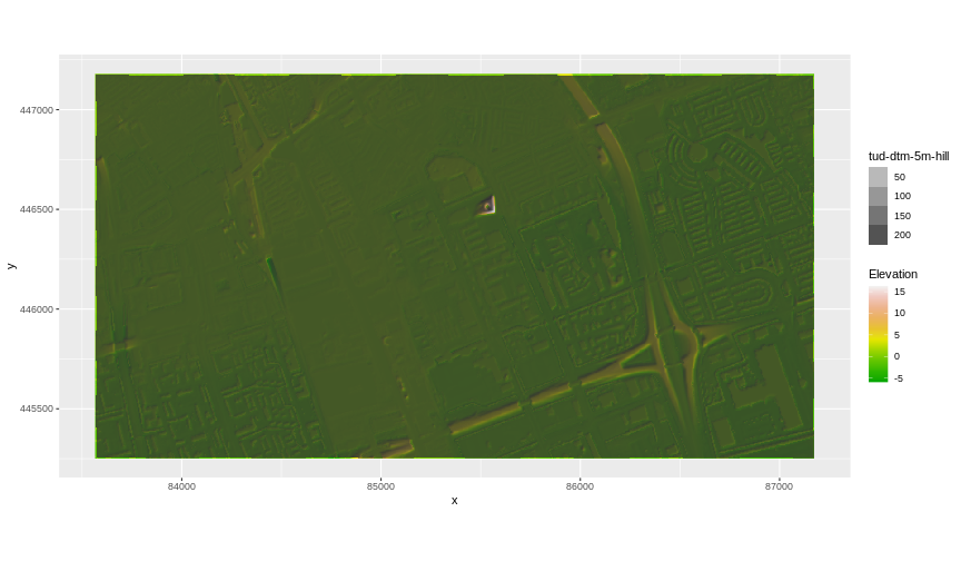
We have now successfully draped the Digital Terrain Model on top of our hillshade to produce a nice looking, textured map!
Key Points
- In order to plot two raster data sets together, they must be in the same CRS.
- Use the
project()function to convert between CRSs.