Import and Visualise OSM Data
Last updated on 2025-07-02 | Edit this page
Overview
Questions
- How to import and work with vector data from OpenStreetMap?
Objectives
After completing this episode, participants should be able to…
- Import OSM vector data from the API
- Select and manipulate OSM vector data
- Visualise and map OSM Vector data
- Use Leaflet for interactive mapping
What is OpenStreetMap?
OpenStreetMap (OSM) is a collaborative project which aims at mapping the world and sharing geospatial data in an open way. Anyone can contribute, by mapping geographical objects they encounter, by adding topical information on existing map objects (their name, function, capacity, etc.), or by mapping buildings and roads from satellite imagery.
This information is then validated by other users and eventually added to the common “map” or information system. This ensures that the information is accessible, open, verified, accurate and up-to-date.
The result looks like this: 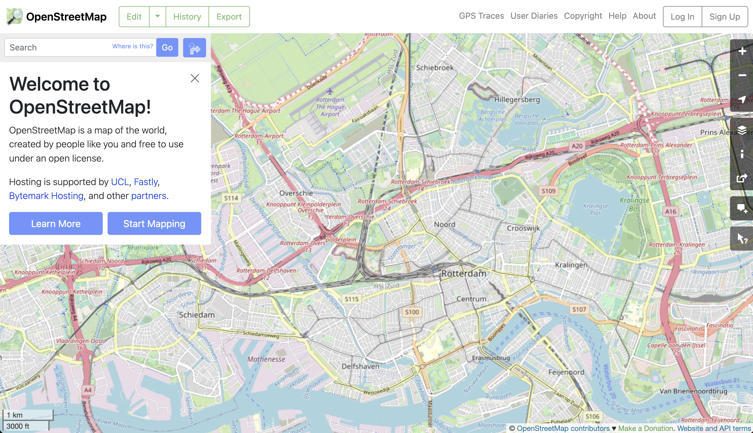
The geospatial data underlying this interface is made of geometrical objects (i.e. points, lines, polygons) and their associated tags (#building #height, #road #secondary #90kph, etc.).
How to extract geospatial data from OpenStreetMap?
R
library(tidyverse)
library(sf)
assign("has_internet_via_proxy", TRUE, environment(curl::has_internet))
Bounding box
The first thing to do is to define the area within which you want to
retrieve data, aka the bounding box. This can be defined easily
using a place name and the package osmdata to access the
free Nominatim API provided by OpenStreetMap.
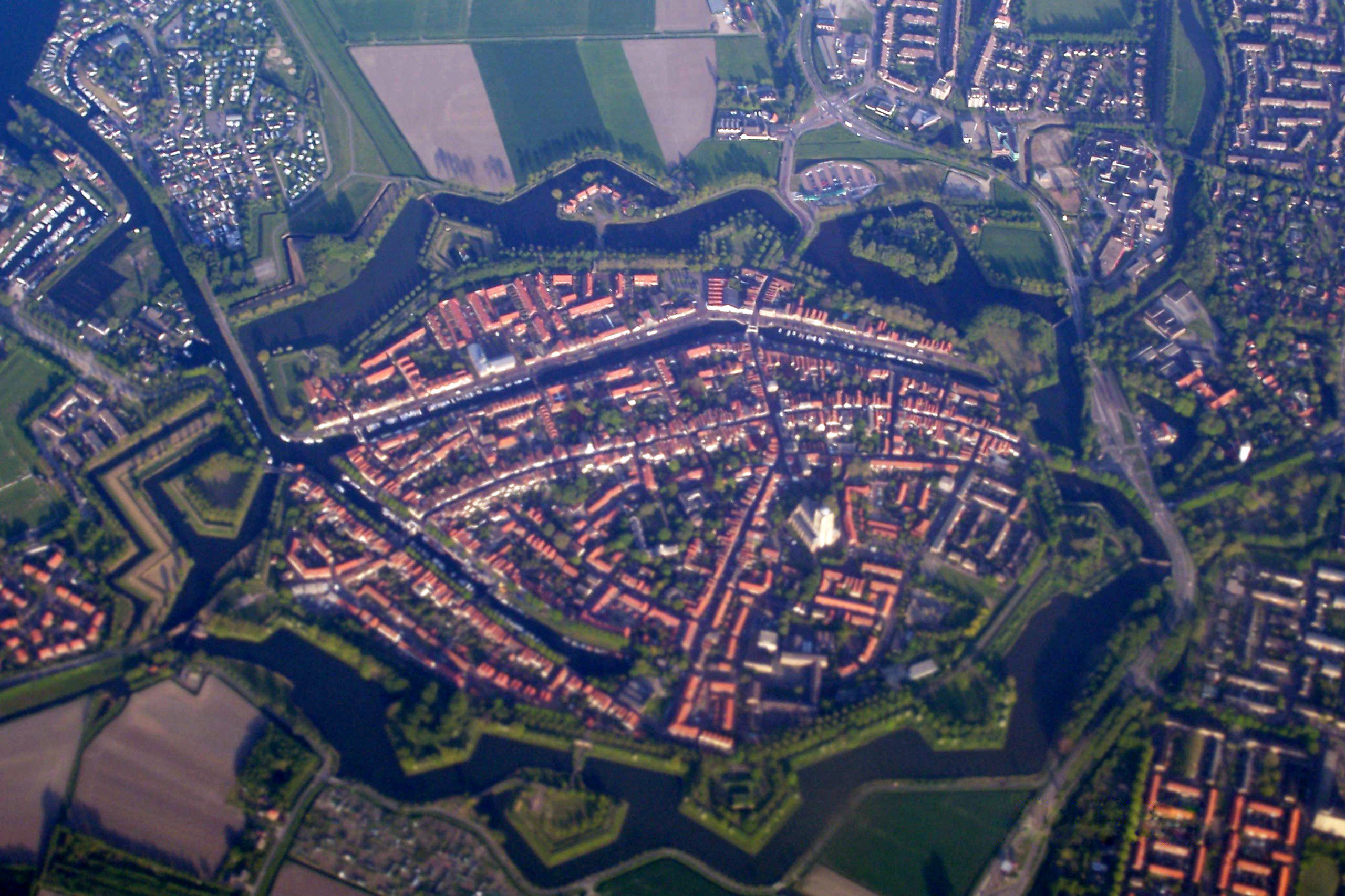
We are going to look at Brielle together.
Callout
Beware that downloading and analysing the data for larger cities might be long, slow and cumbersome on your machine. If you choose another location to work with, please try to choose a city of similar size!
We first geocode our spatial text search and extract the
corresponding bounding box (getbb).
R
library(osmdata)

bb <- osmdata::getbb("Brielle")
bb
OUTPUT
        min       max
x  4.135294  4.229222
y 51.883500 51.931410A word of caution
There might be multiple responses from the API query, corresponding to different objects at the same location, or different objects at different locations. For example: Brielle (Netherlands) and Brielle (New Jersey)

By default, getbb() from the osmdata
package returns the first item. This means that regardless of the number
of returned locations with the given name, the function will return a
bounding box and it might be that we are not looking for the first item.
We should therefore try to be as unambiguous as possible by adding a
country code or district name.
R
bb <- getbb("Brielle, NL")
bb
OUTPUT
        min       max
x  4.135294  4.229222
y 51.883500 51.931410
Extracting features
A feature in
the OSM language is a category or tag of a geospatial object. Features
are described by general keys (e.g. “building”, “boundary”, “landuse”,
“highway”), themselves decomposed into sub-categories (values) such as
“farm”, “hotel” or “house” for buildings, “motorway”,
“secondary” and “residential” for highway. This determines
how they are represented on the map.
Searching documentation
Let’s say we want to download data from OpenStreetMap and we know
there is a package for it named osmdata, but we don’t know
which function to use and what arguments are needed. Where should we
start?
Let’s check the documentation online:
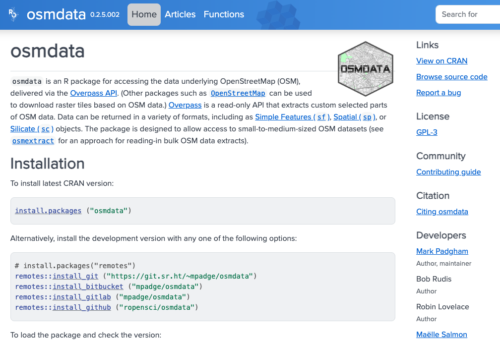
It appears that there is a function to extract features, using the
Overpass API. This function is opq() (for OverPassQuery)
which, in combination with add_osm_feature(), seems to do
the job. However, it might not be crystal clear how to apply it to our
case. Let’s click on the function name in the documentation to find out
more.

On this page we can read about the arguments needed for each
function: a bounding box for opq() and some
key and value for
add_osm_feature(). Thanks to the examples provided, we can
assume that these keys and values correspond to different levels of tags
from the OSM classification. In our case, we will keep it at the first
level of classification, with “buildings” as key, and no
value. We also see from the examples that another function is needed
when working with the sf package:
osmdata_sf(). This ensures that the type of object is
suited for sf. With these tips and examples, we can write
our feature extraction function as follows:
R
x <- opq(bbox = bb) |>
  add_osm_feature(key = "building") |>
  osmdata_sf()
Structure of objects
What is this x object made of? It is a data frame of all
the buildings contained in the bounding box, which gives us their OSM
id, their geometry and a range of attributes, such as their name,
building material, building date, etc. The completion level of this data
frame depends on user contributions and open resources. Here, for
instance, the national BAG dataset was
used and it is quite complete, but that is different in other
countries.
R
str(x$osm_polygons)
OUTPUT
Classes 'sf' and 'data.frame':	10749 obs. of  63 variables:
 $ osm_id                                    : chr  "40267783" "40267787" "40267791" "40267800" ...
 $ name                                      : chr  NA NA NA NA ...
 $ addr:city                                 : chr  NA NA NA NA ...
 $ addr:housenumber                          : chr  NA NA NA NA ...
 $ addr:postcode                             : chr  NA NA NA NA ...
 $ addr:street                               : chr  NA NA NA NA ...
 $ alt_name                                  : chr  NA NA NA NA ...
 $ amenity                                   : chr  NA NA NA NA ...
 $ architect                                 : chr  NA NA NA NA ...
 $ bridge:support                            : chr  NA NA NA NA ...
 $ building                                  : chr  "yes" "yes" "yes" "yes" ...
 $ building:levels                           : chr  NA NA NA NA ...
 $ building:material                         : chr  NA NA NA NA ...
 $ building:name                             : chr  NA NA NA NA ...
 $ camp_site                                 : chr  NA NA NA NA ...
 $ capacity                                  : chr  NA NA NA NA ...
 $ colour                                    : chr  NA NA NA NA ...
 $ construction                              : chr  NA NA NA NA ...
 $ content                                   : chr  NA NA NA NA ...
 $ cuisine                                   : chr  NA NA NA NA ...
 $ dance:teaching                            : chr  NA NA NA NA ...
 $ denomination                              : chr  NA NA NA NA ...
 $ description                               : chr  NA NA NA NA ...
 $ diameter                                  : chr  NA NA NA NA ...
 $ fixme                                     : chr  NA NA NA NA ...
 $ generator:method                          : chr  NA NA NA NA ...
 $ generator:source                          : chr  NA NA NA NA ...
 $ golf                                      : chr  NA NA NA NA ...
 $ height                                    : chr  NA NA NA NA ...
 $ heritage                                  : chr  NA NA NA NA ...
 $ heritage:operator                         : chr  NA NA NA NA ...
 $ historic                                  : chr  NA NA NA NA ...
 $ image                                     : chr  NA NA NA NA ...
 $ layer                                     : chr  NA NA NA NA ...
 $ leisure                                   : chr  NA NA NA NA ...
 $ level                                     : chr  NA NA NA NA ...
 $ location                                  : chr  NA NA NA NA ...
 $ man_made                                  : chr  "storage_tank" "storage_tank" "storage_tank" "storage_tank" ...
 $ material                                  : chr  NA NA NA NA ...
 $ natural                                   : chr  NA NA NA NA ...
 $ old_name                                  : chr  NA NA NA NA ...
 $ operator                                  : chr  NA NA NA NA ...
 $ operator:wikidata                         : chr  NA NA NA NA ...
 $ power                                     : chr  NA NA NA NA ...
 $ rce:ref                                   : chr  NA NA NA NA ...
 $ ref                                       : chr  "`0903" "F-51" "F-61" "F-7" ...
 $ ref:bag                                   : chr  NA NA NA NA ...
 $ ref:bag:old                               : chr  NA NA NA NA ...
 $ ref:rce                                   : chr  NA NA NA NA ...
 $ religion                                  : chr  NA NA NA NA ...
 $ roof:levels                               : chr  NA NA NA NA ...
 $ roof:shape                                : chr  NA NA NA NA ...
 $ seamark:shoreline_construction:category   : chr  NA NA NA NA ...
 $ seamark:shoreline_construction:water_level: chr  NA NA NA NA ...
 $ seamark:type                              : chr  NA NA NA NA ...
 $ source                                    : chr  NA NA NA NA ...
 $ source:date                               : chr  NA NA NA NA ...
 $ start_date                                : chr  NA NA NA NA ...
 $ tourism                                   : chr  NA NA NA NA ...
 $ website                                   : chr  NA NA NA NA ...
 $ wikidata                                  : chr  NA NA NA NA ...
 $ wikipedia                                 : chr  NA NA NA NA ...
 $ geometry                                  :sfc_POLYGON of length 10749; first list element: List of 1
  ..$ : num [1:14, 1:2] 4.22 4.22 4.22 4.22 4.22 ...
  .. ..- attr(*, "dimnames")=List of 2
  .. .. ..$ : chr [1:14] "485609017" "485609009" "485609011" "485609018" ...
  .. .. ..$ : chr [1:2] "lon" "lat"
  ..- attr(*, "class")= chr [1:3] "XY" "POLYGON" "sfg"
 - attr(*, "sf_column")= chr "geometry"
 - attr(*, "agr")= Factor w/ 3 levels "constant","aggregate",..: NA NA NA NA NA NA NA NA NA NA ...
  ..- attr(*, "names")= chr [1:62] "osm_id" "name" "addr:city" "addr:housenumber" ...
Mapping
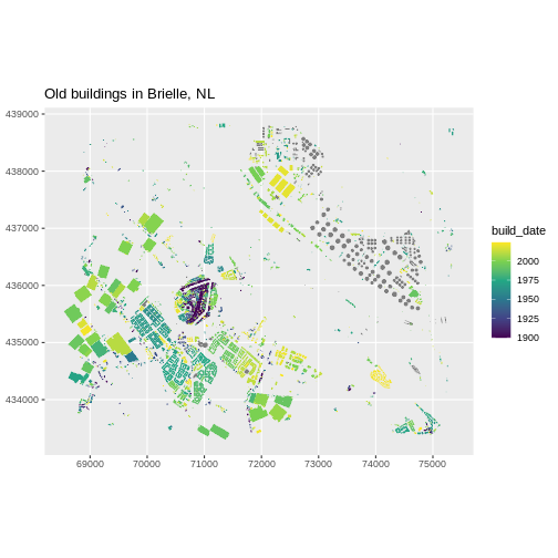
Let’s map the building age of post-1900 Brielle buildings.
Projections
First, we are going to select the polygons and reproject them with the Amersfoort/RD New projection, suited for maps centred on the Netherlands. This code for this projection is: 28992.
R
buildings <- x$osm_polygons |>
  st_transform(crs = 28992)
Visualisation
Then we create a new variable using the threshold at 1900. Every date
before 1900 will be recoded as 1900, so that buildings
older than 1900 will be represented with the same shade.
Then we use the ggplot() function to visualise the
buildings by age. The specific function to represent information as a
map is geom_sf(). The rest works like other graphs and
visualisation, with aes() for the aesthetics.
R
start_date <- as.numeric(buildings$start_date)
buildings$build_date <- if_else(start_date < 1900, 1900, start_date)

ggplot(data = buildings) +
  geom_sf(aes(fill = build_date, colour = build_date)) +
  scale_fill_viridis_c(option = "viridis") +
  scale_colour_viridis_c(option = "viridis") +
  coord_sf(datum = st_crs(28992))
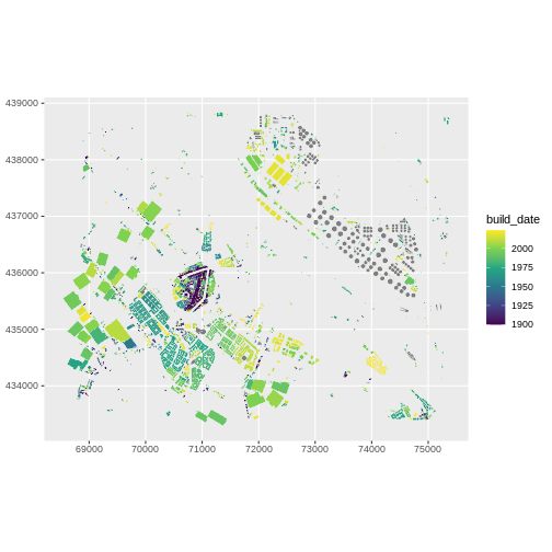
So this reveals the historical centre of Brielle (or the city you chose) and the various urban extensions through time. Anything odd? What? Around the centre? Why these limits / isolated points?
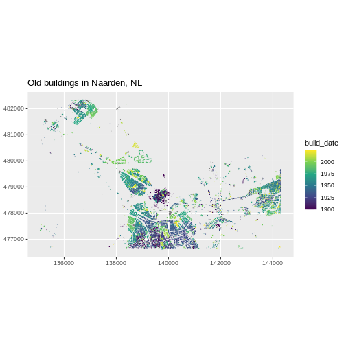
Replicability
We have produced a proof a concept on Brielle, but can we factorise our work to be replicable with other small fortified cities? You can use any of the following cities: Naarden, Geertruidenberg, Gorinchem, Enkhuizen or Dokkum.
We might replace the name in the first line and run everything again. Or we can create a function.
R
extract_buildings <- function(cityname, year = 1900) {
  bb <- getbb(cityname)

  x <- opq(bbox = bb) |>
    add_osm_feature(key = "building") |>
    osmdata_sf()

  buildings <- x$osm_polygons |>
    st_transform(crs = 28992)

  start_date <- as.numeric(buildings$start_date)

  buildings$build_date <- if_else(start_date < year, year, start_date)
  ggplot(data = buildings) +
    geom_sf(aes(fill = build_date, colour = build_date)) +
    scale_fill_viridis_c(option = "viridis") +
    scale_colour_viridis_c(option = "viridis") +
    ggtitle(paste0("Old buildings in ", cityname)) +
    coord_sf(datum = st_crs(28992))
}

# test on Brielle
extract_buildings("Brielle, NL")
R
# test on Naarden
extract_buildings("Naarden, NL")
Going interactive.
Leaflet is an “open-source
JavaScript library for mobile-friendly interactive maps”. It allows
to create interactive maps on which you can zoom, navigate and click for
pop-up information. Within R, there is a corresponding package called
leaflet.
As with ggplot2, you build a leaflet map as a collection
of layers. In this case, you will have a leaflet basemap with tiles, and
one or more layers of shapes (such as points, lines and polygons). You
can also add settings such as the default level of zoom, default
location and content of pop-ups.
The standard structure of a leaflet choropleth map is therefore:
leaflet(data) |> addTiles() |> addPolygons(~variable)
where data is our dataset and variable the
variable we use to colour the polygons. The standard projection used in
Leaflet is WGS84.
- Check out the leaflet package documentation for more information.
Challenge: import an interactive basemap layer under the buildings with ‘Leaflet’ (20min)
For this challenge, you will have to use the Leaflet online
documentation to create an interactive map of the building ages in
Brielle. The underlying data remains the same, but you will use the
leaflet package to make the map interactive (in other words, your
data is the R object buildings and
variable corresponds to start_date).
To do this, you will have to: - Transform the CRS of
buildings into WGS84 - Plot the basemap - Add the tiles of
your choice - Add polygons (the buildings) - Use the
fillColor attribute of these polygons to represent the
build_date variable.
You will find guidance and examples on how to do that in the following links: - Basemap and tiles documentation basemap documentation - Choropleth documentation. Tip: use the examples given in the documentation and replace the variable names where needed. You can also check out the GDCU cheatsheet for relevant leaflet functions.
R
# install.packages("leaflet")
library(leaflet)


buildings2 <- buildings |>
  st_transform(crs = 4326)

# leaflet(buildings2) |>
#  addTiles() |>
#   addPolygons(fillColor = ~colorQuantile("YlGnBu", -build_date)(-build_date))

# For a better visual rendering, try:

leaflet(buildings2) |>
  addProviderTiles(providers$CartoDB.Positron) |>
  addPolygons(
    color = "#444444",
    weight = 0.1,
    smoothFactor = 0.5,
    opacity = 0.2, fillOpacity = 0.8,
    fillColor = ~ colorQuantile("YlGnBu", -build_date)(-build_date),
    highlightOptions = highlightOptions(
      color = "white", weight = 2,
      bringToFront = TRUE
    )
  )
Key Points
- Use the
NominatimandOverpassAPIs within R - Use the
osmdatapackage to retrieve geospatial data - Select features and attributes among OSM tags
- Use the
ggplot,sfandleafletpackages to map data