Basic GIS operations with R and sf
Last updated on 2025-07-02 | Edit this page
Overview
Questions
- How to perform basic GIS operations with the
sfpackage?
Objectives
After completing this episode, participants should be able to…
- Perform geoprocessing operations such as unions, joins and
intersections with dedicated functions from the
sfpackage - Compute the area of spatial polygons
- Create buffers and centroids
- Map and save the results
R
library(tidyverse)
library(sf)
library(osmdata)
library(leaflet)
library(lwgeom)
library(units)
assign("has_internet_via_proxy", TRUE, environment(curl::has_internet))
Why sf for GIS?
As introduced in an
earlier lesson, sf is a package which supports simple
features (sf), “a standardized
way to encode spatial vector data.”. It contains a large set of
functions to achieve all the operations on vector spatial data for which
you might use traditional GIS software: change the coordinate system,
join layers, intersect or unite polygons, create buffers and centroids,
etc. cf. the sf cheatsheet.
Conservation in Brielle, NL
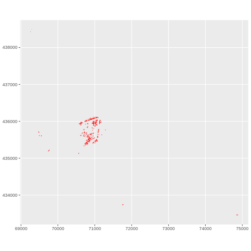
Let’s focus on old buildings and imagine we’re in charge of their conservation. We want to know how much of the city would be affected by a non-construction zone of 100m around pre-1800 buildings.
Let’s select them and see where they are.
R
bb <- osmdata::getbb("Brielle, NL")
x <- opq(bbox = bb) |>
  add_osm_feature(key = "building") |>
  osmdata_sf()
buildings <- x$osm_polygons |>
  st_transform(crs = 28992)


summary(buildings$start_date)
OUTPUT
   Length     Class      Mode
    10749 character character
R
old <- 1800 # year prior to which you consider a building old

buildings$start_date <- as.numeric(buildings$start_date)

old_buildings <- buildings |>
  filter(start_date <= old)

ggplot(data = old_buildings) +
  geom_sf(colour = "red") +
  coord_sf(datum = st_crs(28992))
As conservationists, we want to create a zone around historical buildings where building regulation will have special restrictions to preserve historical buildings.
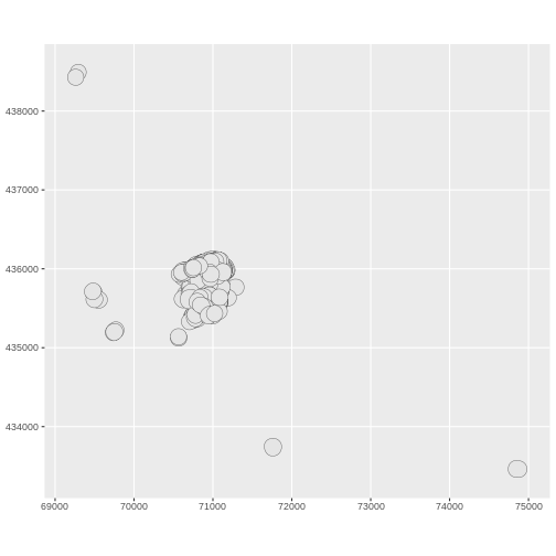
Buffers
Let’s say the conservation zone should be 100 meters. In GIS terms,
we want to create a buffer around polygons. The corresponding
sf function is st_buffer(), with 2 arguments:
the polygons around which to create buffers, and the radius of the
buffer.
R
distance <- 100 # in meters

# First, we check that the "old_buildings" layer projection is measured
# in meters:
st_crs(old_buildings)
OUTPUT
Coordinate Reference System:
  User input: EPSG:28992
  wkt:
PROJCRS["Amersfoort / RD New",
    BASEGEOGCRS["Amersfoort",
        DATUM["Amersfoort",
            ELLIPSOID["Bessel 1841",6377397.155,299.1528128,
                LENGTHUNIT["metre",1]]],
        PRIMEM["Greenwich",0,
            ANGLEUNIT["degree",0.0174532925199433]],
        ID["EPSG",4289]],
    CONVERSION["RD New",
        METHOD["Oblique Stereographic",
            ID["EPSG",9809]],
        PARAMETER["Latitude of natural origin",52.1561605555556,
            ANGLEUNIT["degree",0.0174532925199433],
            ID["EPSG",8801]],
        PARAMETER["Longitude of natural origin",5.38763888888889,
            ANGLEUNIT["degree",0.0174532925199433],
            ID["EPSG",8802]],
        PARAMETER["Scale factor at natural origin",0.9999079,
            SCALEUNIT["unity",1],
            ID["EPSG",8805]],
        PARAMETER["False easting",155000,
            LENGTHUNIT["metre",1],
            ID["EPSG",8806]],
        PARAMETER["False northing",463000,
            LENGTHUNIT["metre",1],
            ID["EPSG",8807]]],
    CS[Cartesian,2],
        AXIS["easting (X)",east,
            ORDER[1],
            LENGTHUNIT["metre",1]],
        AXIS["northing (Y)",north,
            ORDER[2],
            LENGTHUNIT["metre",1]],
    USAGE[
        SCOPE["Engineering survey, topographic mapping."],
        AREA["Netherlands - onshore, including Waddenzee, Dutch Wadden Islands and 12-mile offshore coastal zone."],
        BBOX[50.75,3.2,53.7,7.22]],
    ID["EPSG",28992]]
R
# then we use `st_buffer()`
buffer_old_buildings <-
  st_buffer(x = old_buildings, dist = distance)

ggplot(data = buffer_old_buildings) +
  geom_sf() +
  coord_sf(datum = st_crs(28992))
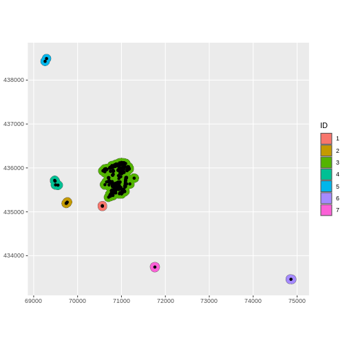
Union
Now, we have a lot of overlapping buffers. We would rather create a
unique conservation zone rather than overlapping ones in that case. So
we have to fuse the overlapping buffers into one polygon. This operation
is called union and the corresponding function is
st_union().
R
single_old_buffer <- st_union(buffer_old_buildings) |>
  st_cast(to = "POLYGON") |>
  st_as_sf()

single_old_buffer <- single_old_buffer |>
  mutate("ID" = as.factor(seq_len(nrow(single_old_buffer)))) |>
  st_transform(crs = 28992)
We also use st_cast() to explicit the type of the
resulting object (POLYGON instead of the default
MULTIPOLYGON) and st_as_sf() to transform the
polygon into an sf object. With this function, we ensure
that we end up with an sf object, which was not the case
after we forced the union of old buildings into a POLYGON
format.
We create unique IDs to identify the new polygons.
Centroids
For the sake of visualisation speed, we would like to represent
buildings by a single point (for instance: their geometric centre)
rather than their actual footprint. This operation means defining their
centroid and the corresponding function is
st_centroid().
R
# s2 works with geographic projections, so to calculate centroids in projected
# CRS units (meters), we need to disable it.
sf::sf_use_s2(FALSE)

centroids_old <- st_centroid(old_buildings) |>
  st_transform(crs = 28992)

ggplot() +
  geom_sf(data = single_old_buffer, aes(fill = ID)) +
  geom_sf(data = centroids_old) +
  coord_sf(datum = st_crs(28992))
Intersection & join
Now, we would like to distinguish conservation areas based on the
number of historic buildings they contain. In GIS terms, we would like
to know how many centroids each fused buffer polygon contains. This
operation means intersecting the layer of polygons with the
layer of points and the corresponding function is
st_intersection(). We then need to join the
aggregated number of centroids with the original layer, using a spatial
left join. The corresponding function is
st_join(., left=T).
R
centroids_buffers <-
  st_intersection(centroids_old, single_old_buffer) |>
  mutate(n = 1)

centroid_by_buffer <- centroids_buffers |>
  group_by(ID) |>
  summarise(n_buildings = n())

single_buffer <- single_old_buffer |>
  st_join(centroid_by_buffer, left = TRUE)

ggplot() +
  geom_sf(data = single_buffer, aes(fill = n_buildings)) +
  scale_fill_viridis_c(
    alpha = 0.8,
    begin = 0.6,
    end = 1,
    direction = -1,
    option = "B"
  ) +
  coord_sf(datum = st_crs(28992))
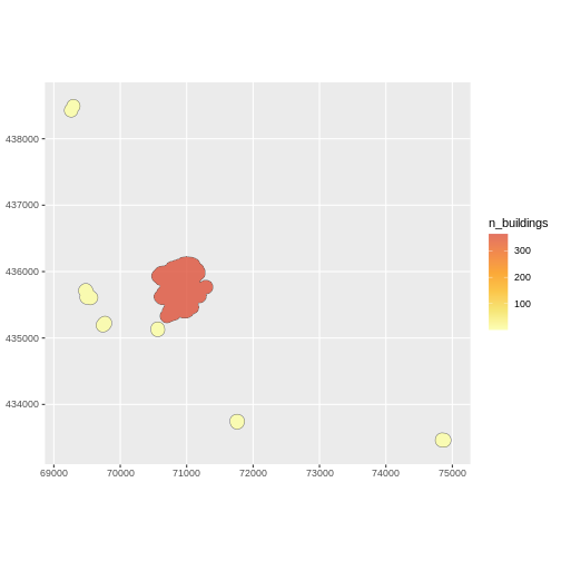
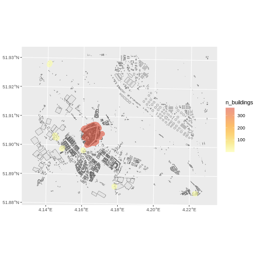
Maps of the number of buildings per zone:
Let’s map this layer over the initial map of individual buildings.
R
ggplot() +
  geom_sf(data = buildings) +
  geom_sf(data = single_buffer, aes(fill = n_buildings), colour = NA) +
  scale_fill_viridis_c(
    alpha = 0.6,
    begin = 0.6,
    end = 1,
    direction = -1,
    option = "B"
  )
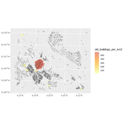
Calculating area and density of spatial features
In our analysis, we have a large number of pre-war buildings, and the buffer zones we’re using are quite broad. As a result, the total count of old buildings within these zones doesn’t provide us with the most meaningful insight. To make our analysis more useful, we should calculate the density of pre-war buildings within each buffer zone. This will help us better understand how these buildings are distributed across the area, providing more relevant and actionable information for our project.
R
single_buffer$area <- st_area(single_buffer) |>
  set_units("km^2")

single_buffer$old_buildings_per_km2 <-
  as.numeric(single_buffer$n_buildings / single_buffer$area)

ggplot() +
  geom_sf(data = buildings) +
  geom_sf(data = single_buffer,
          aes(fill=old_buildings_per_km2),
          colour = NA) +
  scale_fill_viridis_c(
    alpha = 0.6,
    begin = 0.6,
    end = 1,
    direction = -1,
    option = "B"
  )
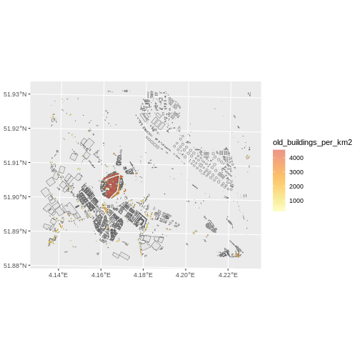
Challenge: Conservation rules have changed.
The historical threshold now applies to all pre-war buildings, but the distance to these building is reduced to 10m. Can you map the density of all buildings per 10m fused buffer?
R
old <- 1939
distance <- 10

# select
old_buildings <- buildings |>
  filter(start_date <= old)

# buffer
buffer_old_buildings <- st_buffer(old_buildings, dist = distance)

# union
single_old_buffer <- st_union(buffer_old_buildings) |>
  st_cast(to = "POLYGON") |>
  st_as_sf()

single_old_buffer <- single_old_buffer |>
  mutate("ID" = seq_len(nrow(single_old_buffer))) |>
  st_transform(single_old_buffer, crs = 4326)

# centroids
centroids_old <- st_centroid(old_buildings) |>
  st_transform(crs = 4326)

# intersection & join
centroids_buffers <-
  st_intersection(centroids_old, single_old_buffer)

centroid_by_buffer <- centroids_buffers |>
  group_by(ID) |>
  summarise(n_buildings = n())

single_buffer <- single_old_buffer |>
  st_join(centroid_by_buffer, left = TRUE)

single_buffer$area <- st_area(single_buffer) |>
  set_units(km^2)
single_buffer$old_buildings_per_km2 <-
  as.numeric(single_buffer$n_buildings / single_buffer$area)

 ggplot() +
   geom_sf(data = buildings) +
   geom_sf(data = single_buffer,
           aes(fill=old_buildings_per_km2),
           colour = NA) +
   scale_fill_viridis_c(
     alpha = 0.6,
     begin = 0.6,
     end = 1,
     direction = -1,
     option = "B"
   )
Key Points
- Use the
st_*functions fromsffor basic GIS operations - Perform unions, joins and intersection operations
- Compute the area of spatial polygons with
st_area()