Tips
When instructing, repeat 3 times:
- talk about the process
- show how it is done
- instruct the participants to do it themselves
Give clear indicators of when learners should be looking at the projector screen, the instructor, or their own laptop (or combination).
Introduction
After warm-up, go through the 3 ML examples:
-
You are trying to understand how temperature affects the speed of embryo development in mice. After running an experiment where you record developmental milestones in mice at various temperatures, you run a linear regression on the results to see what the overall trend is. You use the regression results to predict how long certain developmental milestones will take at temperatures you’ve not tested.
This is machine learning There is a model, the linear regression, which is learning from instances and being used for prediction. Even though a linear regression is simple, when used in this way it is machine learning
-
You want to create a guide for which statistical test should be used in biological experiments. You hand-write a decision tree based on your own knowledge of statistical tests. You create an electronic version of the decision tree which takes in features of an experiment and outputs a recommended statistical test.
While this example contains a decision tree, which is used as a classifier, there is no learning from data. The decision tree is instead being created by hand. This is not machine learning.
-
You are annoyed when your phone rings out loud, and decide to try to teach it to only use silent mode. Whenever it rings, you throw the phone at the floor. Eventually, it stops ringing. “It has learned. This is machine learning,” you think to yourself.
This example appears to contain instances and change with experience, but lacks a model. There is no way to apply anything to future data. This is not machine learning.
T cells
Overall timing:
- Introduce Data: ~3 Min
- ML Workflow:
- Preprocessing: 7 min
- Data split: 15 min
- Training: 10 min
- Testing then predicting: 5 min
- Remaining 5 min - software issues, questions, wiggle room
Notes:
Introduce Data:
Pretty straightforward, just introduce the task and maybe note how we can see differences but it’s difficult and time consuming. Benefits of machine learning for this task: rapidly classify many new cells in real time on a microscopy to sort them.
ML Workflow:
Preprocessing:
Here is where it might be good to actually open up the .csv file and show what it looks like raw. Make a note of data terminology here, things like class, sample, instance, etc. Talk about how the size and intensity features were made, how outliers have to be considered, and where in the software to note various stats like the features, number of samples, etc. Note that data preprocessing is very field specific. For the T cells, Cell Profiler was used for preprocessing to extract features. Some cell images were also removed because they were red blood cells, not T cells.
Data splitting:
Define and give a basic definition of the data split. Currently the lesson uses the analogy of a student cheating on a test. Validation set is like a practice test, okay to take it many times. It is also used to tune the model, which may be like a student adusting their studying strategy. Generally first introduce the idea of needing to have a test set, then introduce the concept of needing to further split the data so we can try things out. The idea of this workflow as an experiment, where we are trying to simulate finding new data we want to use the model on, can be a helpful way to frame this concept as well. The validation set split allows us to experiment as much as we want with changing the model and seeing how it affects performance without ever accidentally cheating and peeking at the test answers, the testing set.
Data leakage scenarios:
These notes are just guides to how to talk about each of the 3 scenarios. Feel no need to follow them exactly. Make sure to do the polls for each scenario.
-
We created a decision tree model to predict whether the compound would inhibit cell growth. We trained the model on the 48 available instances, and found that the decision tree was able to predict those instances with an accuracy of 0.96. Thus, the decision tree is high performing on this task.
This is the improper usage of data. Clues that can lead us to this conclusion are that there is no mention of splitting the data between a training set and a testing set. The only information that is provided is that the accuracy was on the same instances that the model was trained with. What we need to look for is whether or not the result of the experiment tells us how the model would perform on new data we collect The model already saw whether or not each of these compounds inhibits cell growth. So the model already knows the answer to this problem for these 48 instances. It’s going to do better on these than it would on other instances that it hasn’t seen the right answer to This accuracy value is not representative of what would be gotten with new data.
-
We trained 36 different models, each using a different combination of hyperparameters. We trained each model on 80% of the data, withholding 20% of the data to test each model. We present the highest performing model here to show the effectiveness of machine learning on this task.
In this example, we do see that there is a split between the training set and the testing set. This is better than the last scenario, since a test set was used to test the model. However, the testing set was used to select the best of the 36 models instead of a validation set. Thus, information from the testing set has leaked into creating the model. It could be that the best model just performs best on that particular test set, not in general. The models performance is thus likely inflated.
-
We split the data into training and testing sets of 80% and 20%, and further split the training set into a training and validation set. We trained 200 models on the training data, and chose the best-performing model based on performance on the validation set. After choosing and training the model, we found that the model had an accuracy of 0.93 on the testing set.
This example does not appear to have any data leakage. The data was properly split into a training and validation set, and the best model was chosen without looking at the testing set. Thus, we can trust that the performance on the testing set would represent performance on new data given to the model.
After the scenarios, if there is time talk about cross validation but if there is not just mention the figure as an additional resource.
Training
This is mostly showing how the software works and some terminology.
Mention how hyperparameters work and encourage participants to experiment with them.
If participants seem lively it might be nice to ask participants to post the highest accuracy they can get in the chat. Show difference between training and validation metrics.
Be sure to show and explain the data plot and talk about what a decision boundary is.
Feel free to skip the poll here if it doesn’t feel useful in the moment.
Test and predict
There is not much to do here, just emphasize how the software enforces the train the train test split and note that many people’s performance probably went down a bit. This is also the stage where we could predict on new unlabeled data if we had loaded some. Show how to close and restart the software.
Evaluating a model
Explain confusion matrix, define each of the cells, introduce synonyms for these values and metrics. Describe how different evaluation metrics use and emphasize different parts of the confusion matrix. The metric should match the needs of the domains, which we explore with the scenarios.
Split into breakout rooms of 3-4 participants. ~5 minutes for scenario 1, ~8 minutes for scenario 2. Instructors rotate through breakout rooms.
Scenario 1: Want to minimize FP, cannot afford to test the wrong cell line. Precision can be a good metric that accounts for FP.
Scenario 2: FN are important here, do not want to miss a drug that will be effective. Very many TN if classifier predicts all negative. Avoid metrics that use TN, like accuracy. Recall is a good metric, goal is recover good leads (TP) and can tolerate FP so precision isn’t a major issue. Logistic regression will predict all negative because it cannot learn the correct decision boundary. Check the metrics. Accuracy is still high but other metrics like recall are not. The metrics can be unintuitive because precision and recall consider interacting to be positive, then non-interacting to be positive, then average the two values.
Show the simulated drug discovery dataset in the software. The trained model is very bad, which we see in the Data plot, but the accuracy is still very high because of class imbalance.
Introduce error curves, step through the construction of a precision-recall curve. Explain how the purpose of a curve is to avoid calculating precision and recall metrics a single time, calculate them multiple times. Introduce the concept of confidence, which has not come up previously. Can relate it to the blue and red shading in the data plot in the software. Show where the precision-recall curve is in the ml4bio software.
Trees and overfitting
Identify where decision trees may be used implicitly or explicitly in the real world, like medical decision making. Define tree elements, leaves and root. Can draw a tree to show the correspondence. Use the image of the trained tree to show how they can operate with continuous or discrete features. Reintroduce the idea of hyperparameters as the settings of a classifier, explain the main decision tree hyperparameters (max_depth, min_samples_split, class_weights). Introduce overfitting and why an overfit model is not useful even though it performs very well on the training data, why are decision trees prone to overfitting if we don’t limit the depth or sample size.
After loading dataset and letting participants explore decision tree hyperparamters, explain some of the main conclusions. Explain how the lines in the decision boundary correspond to nodes in the decision tree. Explain how hyperparameters affect the decision boundary. Remind everyone that this is an imbalanced dataset when discussing class weights and accuracy.
Random forests are a good classifier for many real datasets. Define underfitting and remind what overfitting looks like in the regression examples. Define bias and variance, how the fit curves would change if one data point is moved. Amount of training data affects whether a high bias or high variance model is appropriate, complex models require more data to fit well. Draw many squiggly lines on the bias/variance example and show how the average of many high variance models gives a good fit. Random forests subsample data and features.
Cell Profiler T cell dataset shows and example of overfitting with the default decision tree. Decision tree with max depth of 2 or random forest can improve validation performance. Discuss the training and validation performance gap.
Overfitting Continued
Only do this part if we are ahead of schedule.
This introduction is intended to motivate random forests and introduce some foundational ideas in learning theory. The goal of this is to make participants begin to consider why a model succeeds, and how data scientists think about machine learning.
First re-hash overfitting, pointing out the definitions of bias and variance. Emphasize: high bias -> simpler models less subject to change -> less overfitting, more training error high variance -> more complex models more subject to change -> more overfitting, less training error
Now we’re going to draw another plot to highlight the relationship between overfitting and the amount of training data
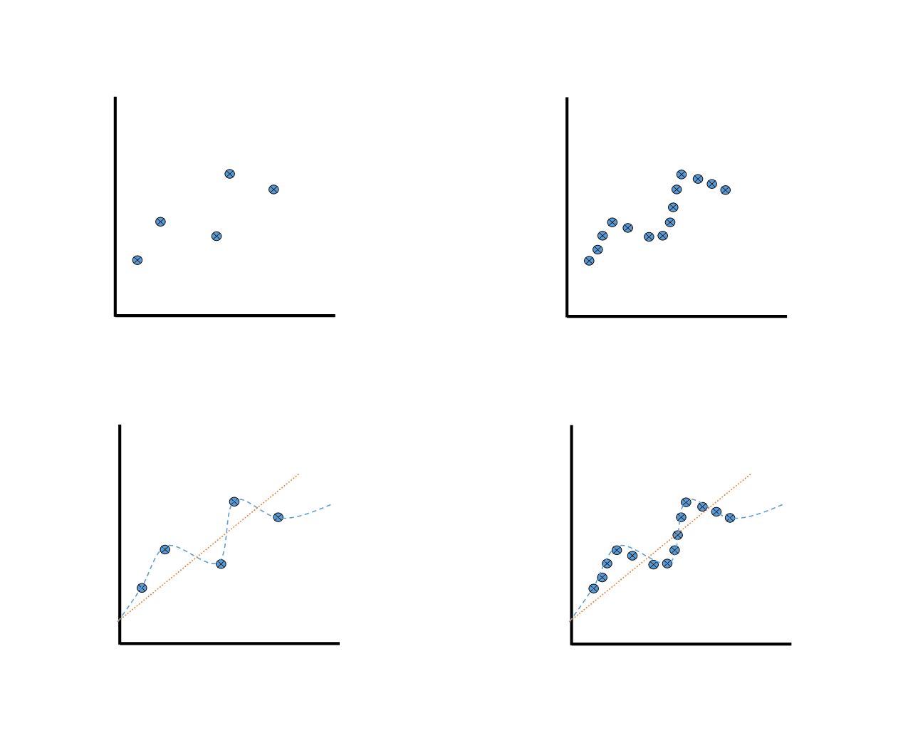
First draw the data plot on the left.
Imagine that it is a st of data for a drug response.
Ask what looks right as a fit line, the straight line or curvy line?
The straight line feels better, as those curves are making a lot of assumptions on the shape of the dose response based on only one data point.
Now add data points so that the plot looks like the plots on the right.
With additional data, we the curvy line looks more appropriate.
Write out the equation for the straight line, y=mx+b (high bias, low variance)
Now write the beginnings of a high-order polynomial for the curvy line, y=ax^9+bx^7+... (low bias, high variance)
Explain how this shows that more data allows us to support more complex models, with a deeper connection to how many parameters the model has.
Random forest motivation
Now that we understand the basics of the bias variance trade-off, we can look at how random forests try to get around it.
Draw the left plot with fewer dots again, and the curvy high variance line
The problem with high variance models is that we’re learning too much to random variation in the training set, new data we collect probably won’t follow the same pattern.
But what if we had a bunch of small training sets, created high-variance models, then averaged them together?
Draw multiple curvy lines with different shapes on the plot
We could average out the error caused by variance across the models, while still maintaining the flexibility and low bias these models give us.
This is the intuition behind random forests, where we use a many trees [a forest of trees] which we setup to have high variance and use them together to choose a final classification.
However, there is still a problem. How do we get enough data for all of these high-variance models? This is where the random in random forests comes in.
We fake having more data by randomly sampling with replacement from the training data. In order to further make sure that our curvy lines are different enough, we also only use a subset of all the features, also chosen randomly, for each tree.
Scenarios
In the following scenarios, which classifier would you choose?
You want to create a model to classify a protein’s subcellular localization (nucleus, mitochondria, plasma membrane, etc.). You have a labeled set of 15,000 human proteins with 237 features for each protein. These features were computationally derived from simulations using protein structure predicting software, and do not have any predefined meaning.
In this scenario, we would probably want to use a random forest. There are a lot of features and data, which means that a random forest’s increased complexity is a good thing here. The features are also not that interpretable, so we’re not too concerned with being able to understand why the model is making certain decisions.
You want to create a model to predict whether or not a species’ conservation status (least concern, endangered, extinct, etc.) will be affected by climate change. You have a labeled dataset of 40 species, with 18 features for each species which have been curated by ecologists. These features include information such as the species’ average size, diet, taxonomic class, migratory pattern, and habitat. You are interested to see which features are most important for predicting a species’ fate.
We have less data in this scenario, so a simpler model might be better. Decision trees are likely the right choice here, especially since we have a very informative, small set of features. We are also interested in being able to interpret the model, which decision trees excel at and random forests can struggle with.
Preparation for day 2
Before ending day 1, ask participants to sign up for a paper to read and discuss on day 2. Pick papers from the Understanding Machine Learning Literature lesson based on their title Can add any papers the participants brought. Use https://padlet.com/ or a similar tool for participants to self-organize into papers so each paper has at least 2 participants.
Logistic Regression, Artificial Neural Networks, and Linear Separability
Introducing logistic regression
Use the TensorFlow Playground example to build intuition about the linear decision boundary of a logistic regression classifier. Modify the feature weights to show how the decision boundary changes. Discuss how this makes logistic regression easy to interpret. Set one weight to 0 to preview the regularization discussion.
Transition to talk about the equations for linear and logistic regression briefly using the network diagram as a guide.
Explain the logistic function shape and purpose.
Work through the toy_data/toy_data_3.csv example.
The example has 3 classes instead of 2 so explain what linear decision boundaries look like with multi-class classification.
Introducing neural networks
Use the TensorFlow Playground examples to show how logistic regression cannot fit the XOR pattern. Adding hidden layers and hidden units with create a neural network that can fit the pattern. Use the spiral example and manually step through a few weight updates to build intuition about how a neural network trains. Discuss how the weights are no longer directly interpretable and require special interpretation techniques. The workshop does not cover gradient descent.
Show the neural network diagram and make the connection to adding more layers and hidden units in TensorFlow Playground.
Work through the toy_data/toy_data_8.csv example.
Discuss why logistic regression cannot fit this multi-class dataset.
Artificial neural networks in practice
Make the connection to the term deep learning. We’re not expected to be able to understand everything ion the robotic surgery arm example. However, we can see that in a modern deep neural network the building blocks are still then same as the simpler models we’ve looked at. We have additional layers which are performing complex tasks on the features of the data to create rich features the final classification layers can predict on.
Classifier selection scenarios
In the following scenarios, which classifier would you choose?
You are interested in learning about how different factors contribute to different water preservation adaptations in plants. You plan to create a model for each of 4 moisture preservation adaptations, and use a dataset of 200 plant species to train each model. You have 15 features for each species, consisting of environmental information such as latitude, average temperature, average rainfall, average sun intensity, etc.
While we can’t be sure, it is likely that each of these features is linear with the class of the data. Things like temperature, rainfall, etc. probably affect moisture preservation adaptations in a single direction. We’re also trying to learn about how factors contribute, not make perfect classifications, so interpretability is important. Therefore, logistic regression is probably the best choice.
You have been tasked with creating a model to predict whether a mole sample is benign or malignant based on gene expression data. Your dataset is a set of 380 skin samples, each of which has expression data for 50 genes believed to be involved in melanoma. It is likely that a combination of genes is required for a mole to be cancerous.
Since it likely takes combinations of mutations to cause a sample to be malignant, the data is probably non-linear. We wouldn’t want to treat the 50 genes independently. Therefore, we should use a neural network for this task.
Regularization
This section is typically skipped unless the lesson is moving more quickly than usual. Refer back to overfitting problems with decision trees and what overfitting means with a logistic regression model. Explain how L1 and L2 penalties reduce the feature weights.
In the simulated_t_cell/simulated_t_cells_1.csv activity, there are a few main takeaways.
When C = 0.001 all feature weights are 0.
Neither feature is used, and all data points are predicted as the same class.
C = 0.07 is the most important value of C.
Here the L1 penalty will set one feature weight to 0 but the L2 penalty will not.
Discuss this difference.
For higher values of C the orientation and steepness of the decision boundary changes, but both features are used.
Understanding machine learning literature
Start by discussing some of the important workflow components to look for when reading a paper: data splitting strategy, type of classifier, how hyperparameters were selected, whether the evaluation metric is appropriate for the dataset. Open the example paper breast cancer susceptibility paper. Narrate going through the paper, looking for the methods section and finding important information like the number of instances, class labels, and features. Highlight the text as this information is located. Try not to jump around the paper too quickly when sharing the screen.
Nested cross validation is used in this paper so explain how that differs from the cross validation we described previously.
Let participants read their papers individually and work on the form for 10 minutes. Then split into breakout rooms organized by paper for 15 minutes. Instructors rotate through the rooms to clarify confusing points or non-traditional workflow decisions. Then return to the entire group and ask participants to share interesting aspects of their papers.
Conclusion
Discuss some of the considerations of machine learning in practice.
Give time to work through the assessment activity. Point out what we modified the paper excerpt, possibly to introduce errors, possibly to correct errors.
Thank participants and encourage them to complete the post-workshop survey to help improve the workshop. Send the survey link by email immediately after the workshop.
Review the References page. Show a few of the extensive ml4bio guides that define the classifiers that were not covered in the workshop (k Nearest Neighbors, Naïve Bayes, Support Vector Machine) and provides a more formal treatment all classifiers. Point out the links to references for next steps, which involves moving from the ml4bio software to code-driven modeling. Software Carpentry teaches basic Python and command line skills, which is one avenue for acquiring the background knowledge needed to tackle the Python-based machine learning tutorials.
Emphasize that the machine learning workflow in the ml4bio software is the same workflow in the example Jupyter notebook that uses Python code. If time permits, open the notebook in Binder to show how it can execute in a web browser and the major workflow steps. Launch the notebook in Binder before the workshop begins so that the image is prepared in advance and the notebook loads quickly.