Logistic Regression, Artificial Neural Networks, and Linear Separability

Overview

Duration: 45 min

Questions

• What is linear separability?

Objectives

• Understand advantages and disadvantages of logistic regression and artificial neural networks

• Distinguish linear and nonlinear classifiers

• Select a linear or nonlinear classifier for a dataset

Logistic Regression

Logistic regression is a classifier that models the probability of a certain label. In the T-cells example, we were classifying whether cells were in the two categories of active or quiescent. Using the logistic regression to predict the whether a cell is active is a binary logistic regression. Everything that applies to the binary classification could be applied to multi-class problems (for example, if there was a third cell state). We will be focusing on the binary classification problem.

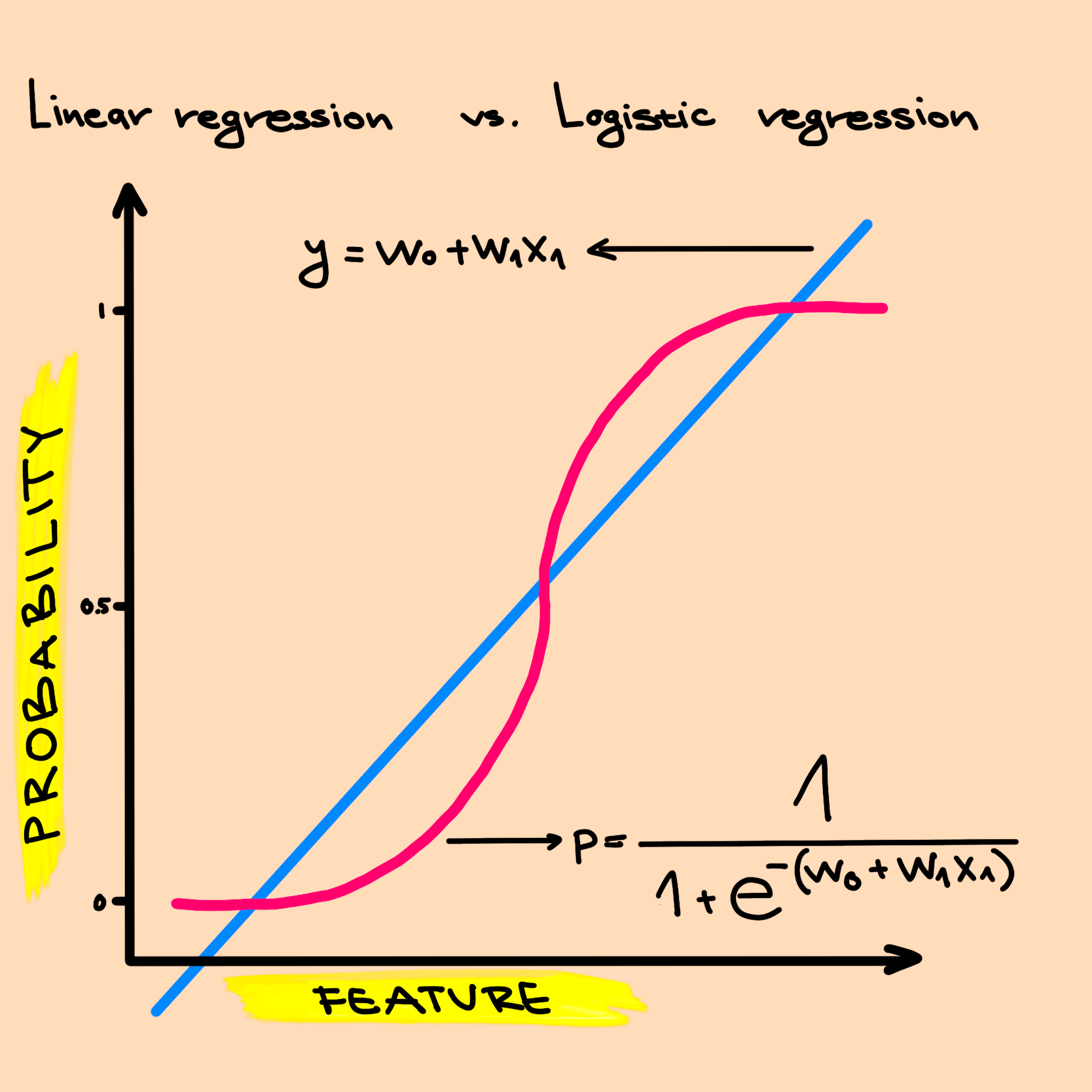
Linear regression vs. logistic regression

We can write the equation for a line as $y=mx+b$, where $x$ is the x-coordinate, $y$ is the y-coordinate, $m$ is the slope, and $b$ is the intercept. We can rename $m$ and $b$ to instead refer to them as feature weights, $y=w_1x+w_0$. Now $w_0$ is the intercept of the line and $w_1$ is the slope of the line. In statistics, for the simple linear regression we write intercept term first $y=w_0+w_1x$.

Definition

Feature weights - determine the importance of a feature in a model.

The intercept term is a constant and is defined as the mean of the outcome when the input $x$ is 0. This interpretation gets more involved with multiple inputs, but that is out of the scope of the workshop. The slope is a feature weight. In the T-cells example, the feature weight is the coefficient for the feature $x$ and it represents the average increase in the confidence the cell is active with a one unit increase in $x$.

When we have multiple features, the linear regression would be $y = w_0 + w_1x_1 + w_2x_2 +…+ w_nx_n$.

What is logistic regression?

Logistic regression returns the probability that a combination of features with weights belongs to a certain class.

In the visual above that compares linear regression to logistic regression, we can see the “S” shaped function is defined by $p = \frac{1}{1+e^{-(w_0+w_1x_1)}}$. The “S” shaped function is the inverse of the logistic function of odds. It guarantees that the outcome will be between 0 and 1. This allows us to treat the outcome as a probability, which also must be between 0 and 1.

Definition

Odds - probability that an event happens divided by probability that an event doesn’t happen.

$odds = \frac{P(event)}{1-P(event)}$

Now, let’s think about the T-cells example. If we focus only on one feature, for example cell size, we can use logistic regression to predict the probability that the cell would be active.

The logistic function of odds is a sum of the weighted features. Each feature is simply multiplied by a weight and then added together inside the logistic function. So logistic regression treats each feature independently. This means that, unlike decision trees, logistic regression is unable to find interactions between features. An example of a feature interaction is if the copy number increase of a certain gene may only affect cell state if another gene is also mutated. This feature independence affects what type of rules logistic regression can learn.

Questions to consider

What could be another example of two features that interact with each other?

An important characteristic of features in logistic regression is how they affect the probability. If the feature weight is positive then the probability of the outcome increases, for example the probability that a T-cell is active increases. If the feature weight is negative then the probability of the outcome decreases, or in our example, the probability that a T-cell is active decreases.

Definition

Linear separability - drawing a line in the plane that separates all the points of one kind on one side of the line, and all the points of the other kind on the other side of the line.

Recall, $y=mx+b$ graphed on the coordinate plane. It is a straight line. $y = w_0 + w_1x_1$ is a straight line. The separating function has the equation $w_0+w_1x_1= 0$. If $w_0+w_1x_1>0$ the T-cell is classified as active, and if $w_0+w_1x_1<0$ the T-cell is classified as quiescent.

Questions to consider

When do you think something is linearly separable?

You can use the TensorFlow Playground website to explore how changing feature weights changes the line in the plane that separates blue and orange points. This example has two features $x_1$ and $x_2$. You can click the the blue lines to modify the weights $w_1$ and $w_2$. Press the play button to automatically train the weights to minimize the number of points that are predicted as the wrong color.

Step 1 Train a Logistic Regression Classifier

Software

Load the toy_data/toy_data_3.csv data set into the software.

This dataset is engineered specifically for the logistic regression classifier.

Linear separability

In this workshop, not all of the hyperparameters in the ml4bio software will be discussed. For those hyperparameters that we don’t cover, we will use the default settings.

Software

Let’s train a logistic regression classifier.

For now use the default hyperparameters.

Questions to consider - Poll

Look at the Data Plot. What do you notice?

Is the data linearly separable?

Logistic regression can also be visualized as a network of features feeding into a single logistic function.

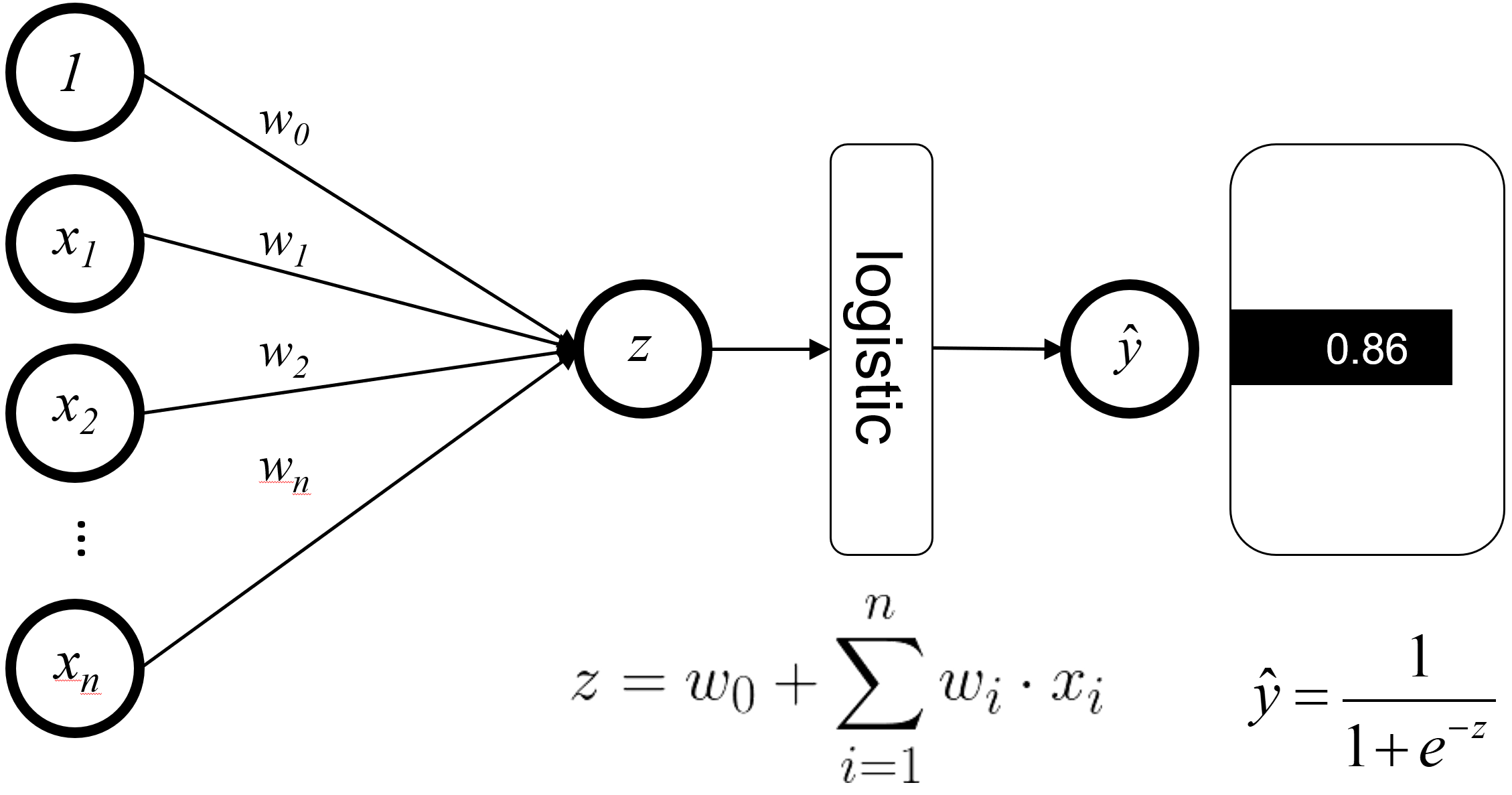
At the logistic function, the connected features are combined and fed into the logistic function to get the classifier’s prediction. In this visualization, we can see that the features never interact with each other until they reach the logistic function, which results in feature independence.

Artificial Neural Networks

An artificial neural network can be viewed as an extension of the logistic regression model, where additional layers of feature interactions are added. These additional layers allow for more complex, non-linear decision boundaries to be learned.

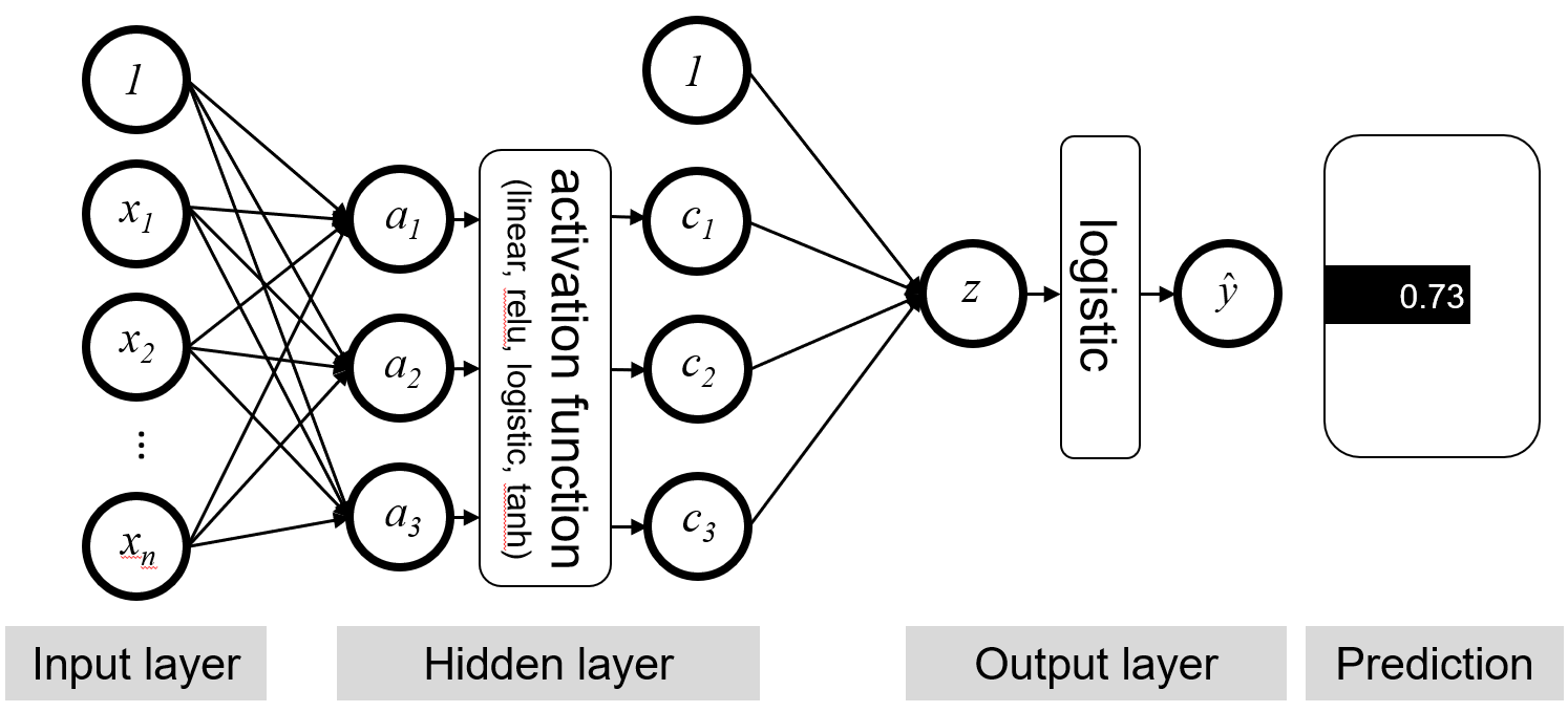
Artificial neural networks have inputs and outputs, just like logistic regression, but have one or more additional layers called hidden layers comprised of hidden units. Hidden layers can contain any number of hidden units. In the neural network diagram, each unit in the input, output, and hidden layers resemble neurons in a human brain, hence the name neural network. The above figure shows a fully connected hidden layer, where every feature interacts with every other feature to form a new value. The new value is created by passing the sum of the weighted feature values into the activation function of the hidden layer. These new values are then fed to the logistic function as opposed to the raw features.

Definitions

Hidden unit - a function in a neural network that takes in values, applies some function to them, and outputs new values to be used in subsequent layer of the neural network.

Hidden layer - a layer of hidden units in a neural network, such as the logistic function.

Activation function - the function used to combine values in a specific layer of a neural network.

You can again use TensorFlow Playground to examine the difference between logistic regression, which has a single logistic function, and a neural network with multiple hidden layers. This example initially attemps to use logistic regression to separate the orange and blue points. Try adding more hidden layers and more neurons in each layer using the play button to train the weights.

This final example has a complicated orange/blue pattern. Press the play button to watch how the neural network can iteratively make small weight updates that reduce the number of mislabeled points.

Step 2 Compare Linear and Nonlinear classifiers

Software

Load the toy_data/toy_data_8.csv data set into the software.

This data set is engineered specifically to demonstrate the difference between linear and nonlinear classifiers.

Train a logistic regression classifier using the default hyperparameters.

Questions to consider

What are the evaluation metrics telling us?

Look at the Data Plot. What do you notice?

Is the data linearly separable?

Software

Now train a neural network on the same data.

Questions to consider

What shape is the decision boundary?

How did the performance of the model change on the validation data?

This example demonstrates that logistic regression performs great with data that is linearly separable. However, with the nonlinear data, more complex models such as artificial neural networks need to be used.

Artificial neural networks in practice

Artificial neural networks with a single hidden layer tend to perform well on simpler data, such as the toy datasets in this workshop.

However artificial neural networks used on more complex data, such as raw image data or protein structure data, typically have much more complex architectures.

For example, below is the architecture of a neural network used to evaluate the skill of robotic surgery arms based on motion captured over time.

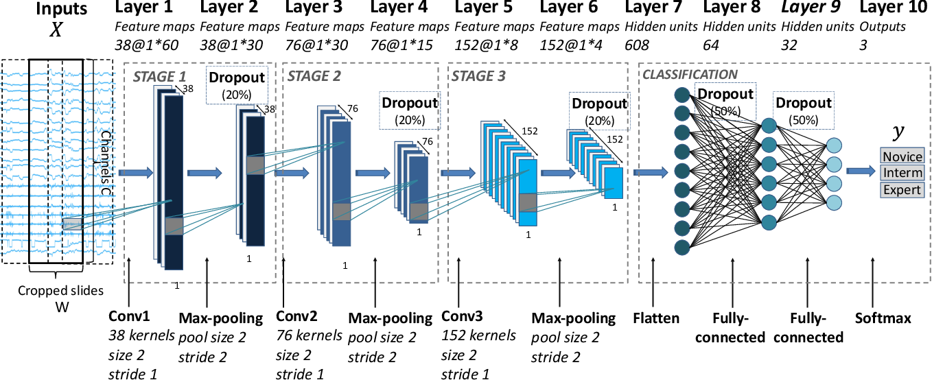
This neural network still consists of hidden layers combined with functions, but contains many specialized layers which perform specific operations on the input features.

Classifier selection scenarios - Poll

In the following scenarios, which classifier would you choose?

1. You are interested in learning about how different factors contribute to water preservation adaptations in plants. You plan to create a model for each of 4 moisture preservation adaptations, where in each model the presence of the moisture preservation adaptation is the class being predicted. You use a dataset of 200 plant species to train each model. You have 15 features for each species, consisting of environmental information such as latitude, average temperature, average rainfall, average sun intensity, etc.

2. You have been tasked with creating a model to predict whether a mole sample is benign or malignant based on gene expression data. Your dataset is a set of 380 skin samples, each of which has expression data for 50 genes believed to be involved in melanoma. It is likely that a combination of genes is required for a mole to be cancerous.

Step 3 Test Regularization Strategies

Regularization

Regularization is used to make sure that our model pays attention only to the important features to avoid overfitting. Previously, we talked about the positive and negative effect a feature and its weight can have on the outcome probability. As with decision trees and random forests, logistic regression can overfit. If we have a complex model with many features, our model might have high variance. Regularization can help us decide how many features are too many or too few. Regularization does not make models fit better on the training data, but it helps with generalizing the pattern to new data.

Definition

Regularization - approaches to make machine learning models less complex in order to reduce overfitting.

Penalty - a regularization strategy that reduces the importance of certain features by adding a cost to the feature weights, which makes the feature weights smaller.

Regularization hyperparameters in the ml4bio software

The most important hyperparameters in the ml4bio software are:

• The regularization penalty can be L1 or L2. Although it is possible to train a logistic regression classifier without regularization, regularization is always used in the ml4bio software. This follows best practices in real applications.
• C is the inverse of the regularization strength. Smaller values of C mean stronger regularization (higher penalties, therefore lower feature weights).

Software

Load the simulated_t_cell/simulated_t_cells_1.csv data set into the software.

This data set is engineered specifically to demonstrate the effects of regularization.

L1 regularization

L1 regularization is also known as Lasso reguralization.

Recall that $x_1, x_2, …, x_n$ are the features, and $w_0, w_1, …, w_n$ are the feature weights. Without regularization, the classifier might fit the training data perfectly, giving certain values to each weight that would lead to overfitting. This model could be very complex and it would generalize poorly on the future data.

L1 regularization prevents overfitting by adding a penalty term and mathematically shrinking (decreasing) some weights. L1 could shrink the weights of less important features all the way to 0, effectively deleting those weights. The corresponding features are then not used at all to make predictions on new data.

L2 Penalty

L2 regularization is also known as ridge reguralization. L2 reguralization makes the weights of less important features to be small values. Unlike L1 regularization, L2 regularization does not necessarily shrink the weights to 0. The higher the value of C, the smaller the feature weights will be.

Recall: C is the inverse of regularization strength. Smaller values of C will shrink more weights and use fewer features to make the prediction.

Software

First, set penalty to ‘L1’. Experiment with C = 0.001, 0.07, 0.1, 0.25, 1.

Next, set penalty to ‘L2’. Experiment with the same values of C.

Questions

What do you observe in the Data Plot? For each value of C, which of the two features seem to influence the decision boundary?

What is the difference between L1 and L2 regularization? (Hint: consider C = 0.07)

How does the decision boundary change as C increases?

L1 can regularize such that one feature’s weight goes to 0. We can see the classifier ignores that feature in its decision boundary.

Break

Let’s take a short break.

Key Points

• Logistic regression is a linear classifier.

• The output of logistic regression is probability of a certain class.

• Artificial neural networks can be viewed as an extension of logistic regression

• Artificial neural networks can have nonlinear decision boundaries