ICA hypothesis testing

Overview

Teaching: 0 min
Exercises: 0 min

Questions

• How can hypothesis testing be performed on ICs instead of scalp signals?

• What tools are available for visualizing ICA ERPs?

• How can we examine ICs across subjects in a group analysis?

Objectives

• Perform data summaries and statistics on ICs in addition to scalp channels

If ICA is able to isolate stationary signals for artifacts it may also be able to isolate stationary cortical sources

How can we identify cortical components?

We can examine which ICs account for specific ERP patterns by comparing the scalp ERPs (with topographies) to the IC ERP envelope plots. In order to accomplish this we can load segmented files one at a time and examine which ICs account for various ERP patterns. Let’s start with sub-s01.

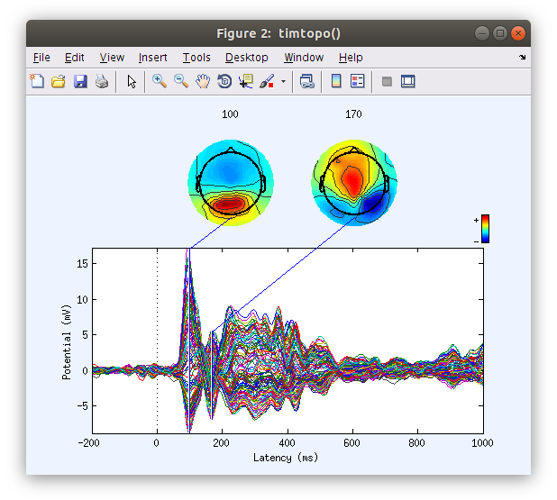
Examine the scalp ERP waveform with topographical maps

By plotting the ERPs of all the channels overlayed one on top of the other we get an understanding of the voltage distribution at each time point along the ERP period. Further by plotting the topographical map at specific time points we see the spatial distribution of the voltages over time. It is important to note here that at the scalp the ERP voltage pattern appears to move around the surface of the scalp.

… Although we select specific time point to plot the topographies when generating the ERP plot, topographies for any time point can be obtained by clicking on the waveforms.

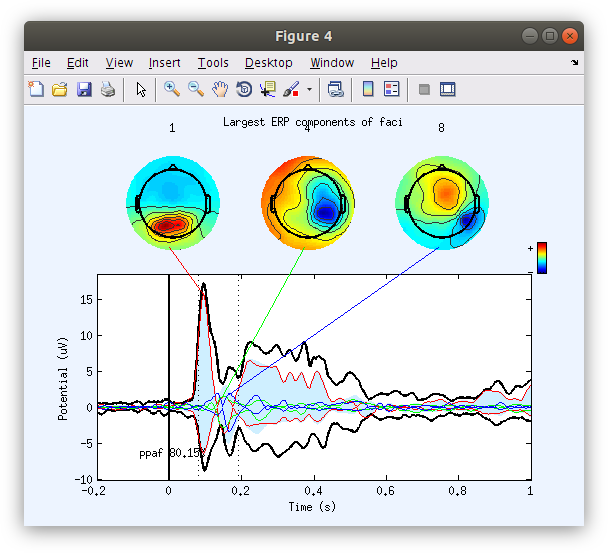
Examine the IC ERP envelope plots with topographical maps

In contrast to plotting scalp channels with topographical maps at specified time points, the IC ERP plot illustrates the IC envelopes (voltage min max at each time point) of each of the top contributing ICs. Each component has a fixed topographical projection and we see that the components vary over time with regards to the percentage of the data that they account for at the scalp (which appears as movement of topographical maps on the scalp surface).

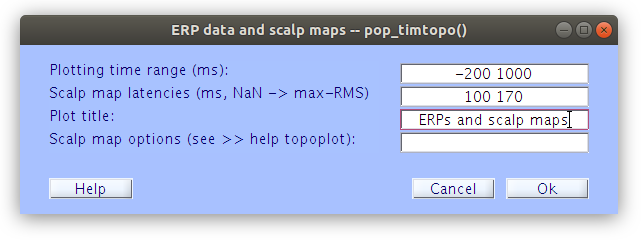
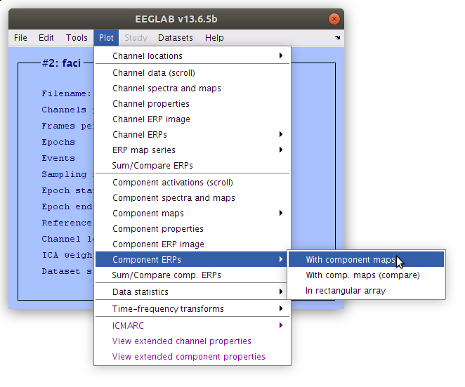
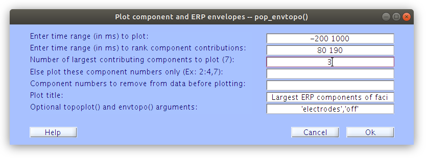
How to generate the ICA plots

Identify the dominant ICs accounting for the P100 and N170 in each recording

In order to analyze ICs they need to be classified. This to say that ICs are not like channels where we can simply choose a medial-occipital site and score it for each participant for example. Each IC has several properties (topographical project, time course of activation, and variance accounted for, etc) that need to be considered before deciding which ICs to analyze. This is both a difficult task, but an important distinction from analyzing scalp signals.

This is a classification list of the IC accounting for the P100 and N170 in the demo data set

1. sub-s01 P100: 1 N170: 4,8
2. sub-s02 P100: 3, 9, 13 N170: 1, 7
3. sub-s03 P100: 2 N170: 3
4. sub-s04 P100: 2 N170: 1
5. sub-s05 P100: 2, 13 N170: 1
6. sub-s06 P100: 1 N170: 4
7. sub-s07 P100: 6, 10 N170: 4, 16
8. sub-s08 P100: 2, 5 N170: 1, 7, 19
9. sub-s09 P100: 21, 22 N170: 1, 6, 13
10. sub-s10 P100: 1, 3, 4 N170: 2

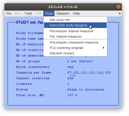
Load a STUDY structure and cluster components

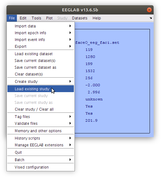
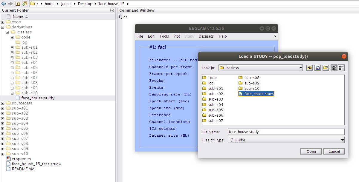
Now that we have IC in our data files and the cortical components of interest have been classified let’s summarise the ERP data again but this time based on the IC signals rather than the scalp signals. We can start by loading the existing face_house.study file which has indexes for all 10 of the participants in the data set.

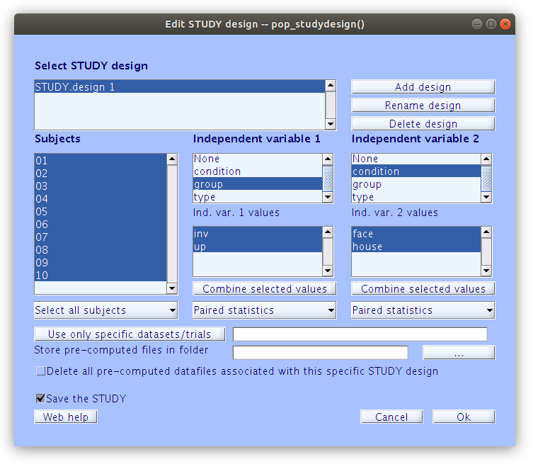
Examine the STUDY Design

Taking a look at the study design we see that we have all 10 participants indexed as well as the two stimulus type independent variables.

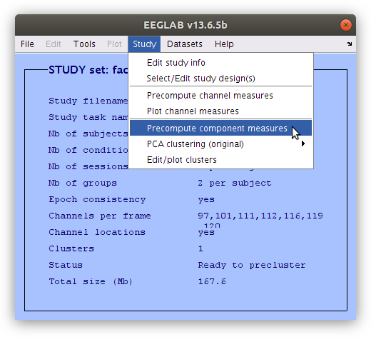
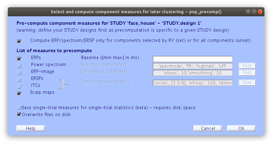
Precompute IC measures

Like we did previously for the scalp signal we need to precompute some measure for the IC, then we can start building summaries of IC activations and cluster the components.

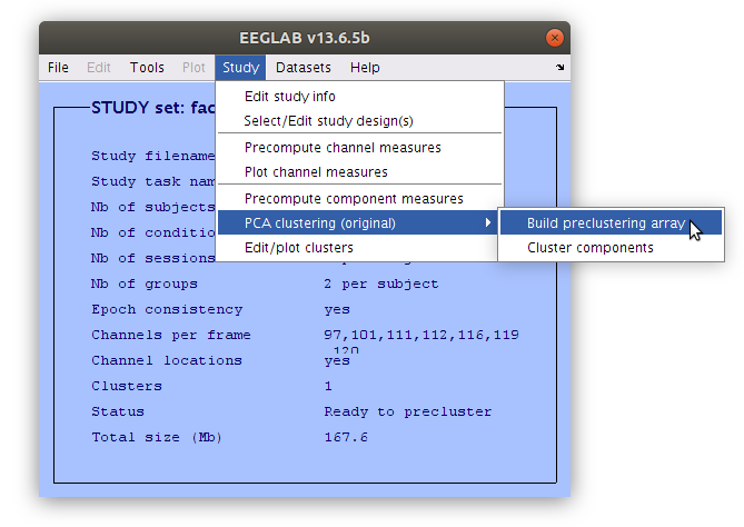
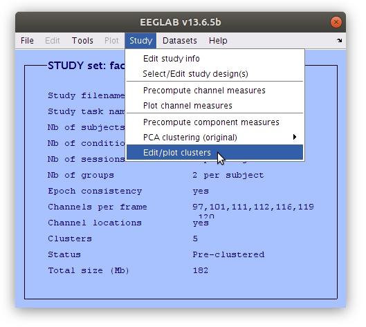
Cluster components

Unlike scalp channels where we can typically use basic parameters to choose which channels are included in an analysis for each subject (e.g. site Oz for each participant, or the maximum channel during a specific time interval for each participant) more complex decisions need to be made about which components are used for each participant. Then we need to cluster those components together to create the signals for the analyses. There are automated ways of doing clustering analyses, but since we have already classified the components that we are interested in we will perform the clustering manually.

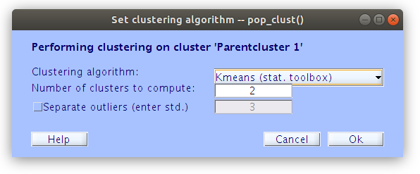
In order to cluster the components manually, we first need to build the basic clustering structures with some minimal parameters.

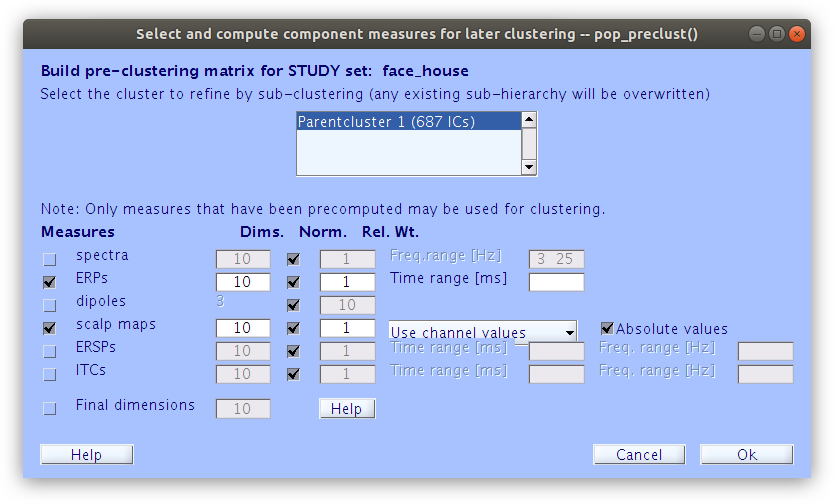
… Once some basic weights are set we can build the initial cluster structure. Note, at this point we are not interested in how EEGLAB clusters the components together, we just need it to build an initial cluster structure so that we can modify it manually.

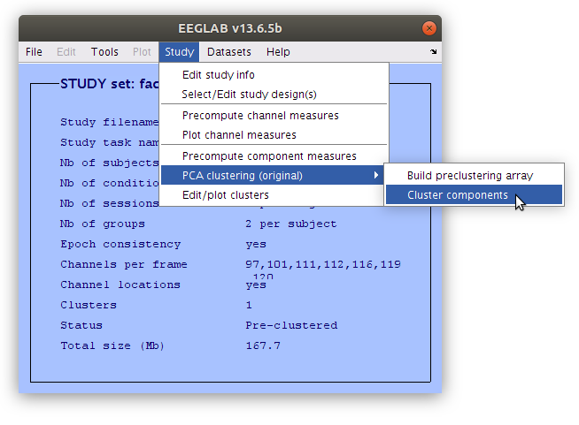
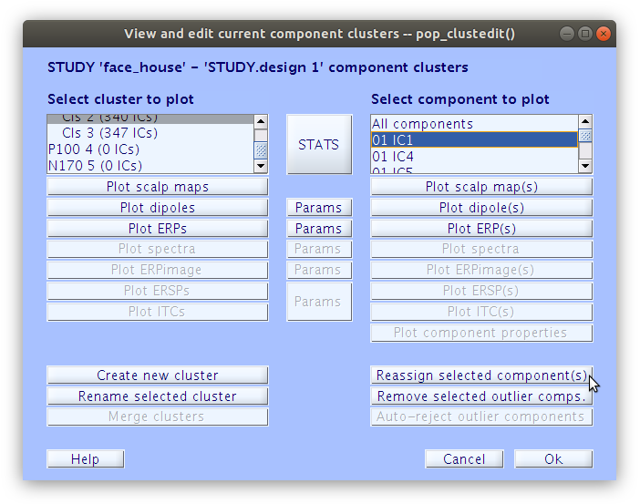
Edit the component cluster.

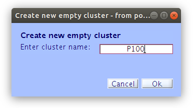
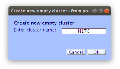
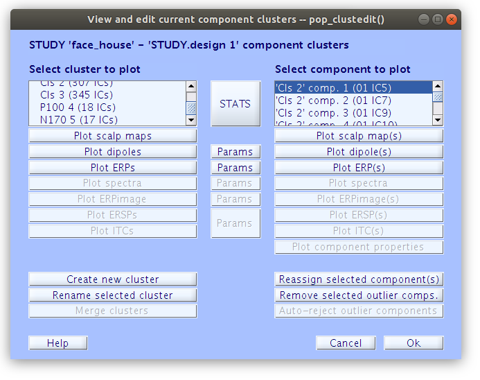
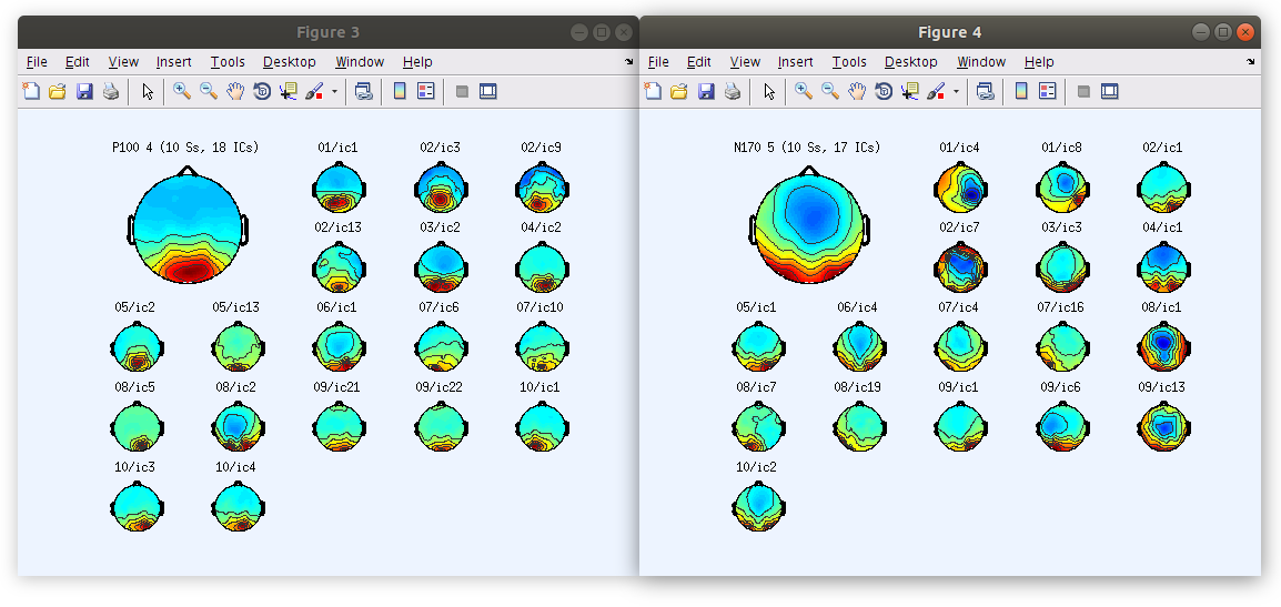
Once the clustering is complete the GUI for viewing and editing the component cluster appears and we can start working with the cluster. We asked EEGLAB to cluster the components into two clusters so now we see that there is a “Parent cluster” (containing all of the components in the study) as well as “Cls 2” and “Cls 3”. We want to add two more clusters, specifically “P100” and “N170” then populate those clusters with component classification decisions that we made earlier.

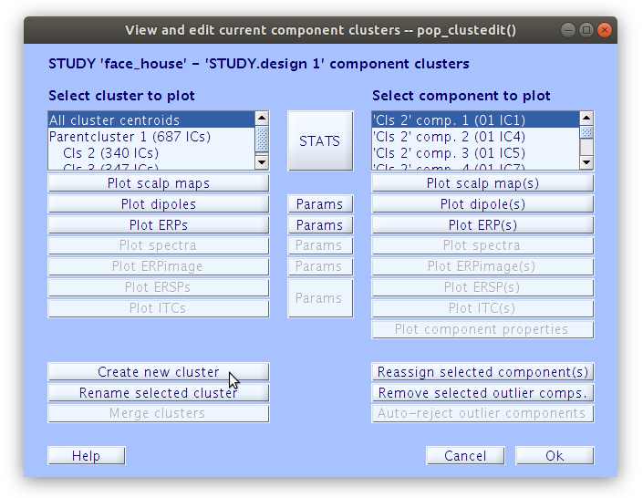
Reassigning components to clusters

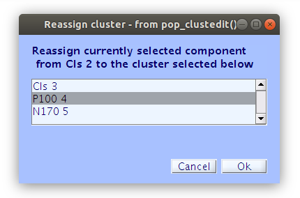
All of the components in the study belong to either “Cls 2” or “Cls 3”. Our goal now is to find all of the components that we classified earlier and reassign them to the new clusters “P100” and “N170” that we created manually. We can do this by selecting a component in the right side list and then clicking “Reassign selected component(s), then selecting the cluster that it should be assigned to.

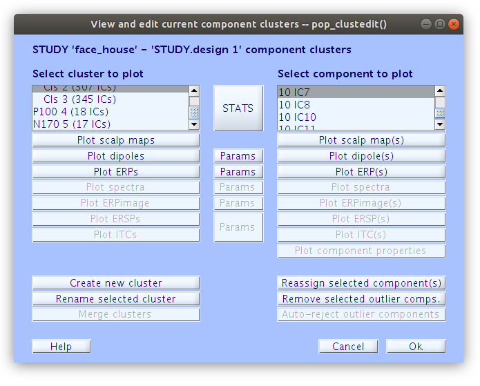
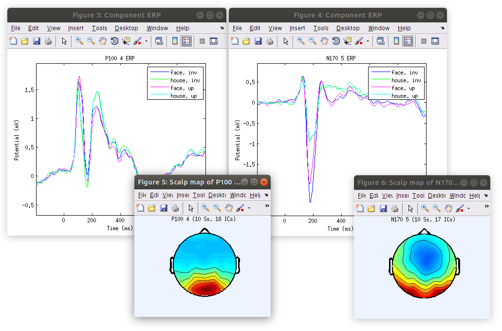
… Once that we reassign all of the components that we have classified as accounting for the P100 and N170 we see that the “P100” cluster contains 18 components and the “N170” cluster contains 17 components.

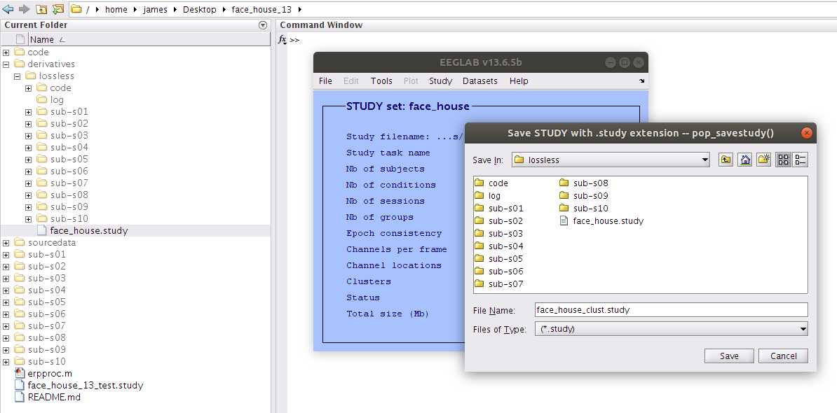
Save the study

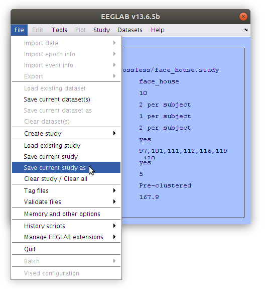
Having committed quite a bit of time to reassigning the components to their cluster we should save a new study file. This will store all of the decisions that have been made so that they can be accessed again later. Save the file with a new name (e.g. face_house_clust.study).

Plot the component cluster summaries

Now that the component clustering is complete we can examine summaries of the components similar to how we did previously with scalp channels.

Key Points

• Increasing the measurement specificity by analysing ICs