Overview

Teaching: 20 min
Exercises: 10 min

Questions

• What does raw Twitter data look like?

• What are some built-in ways of looking at Twitter JSONL data with Jupyter?

• Which pieces of a tweet should I pay attention to?

Objectives

• Getting acquainted with how JSONL looks

• Accessing Twitter data in a human-readable way

Examining a twarc JSONL file

JSONL, Line-oriented JavaScript Object Notation, is frequently used as a data exchange format. It has become super common in the data science field, and you will encounter it frequently.

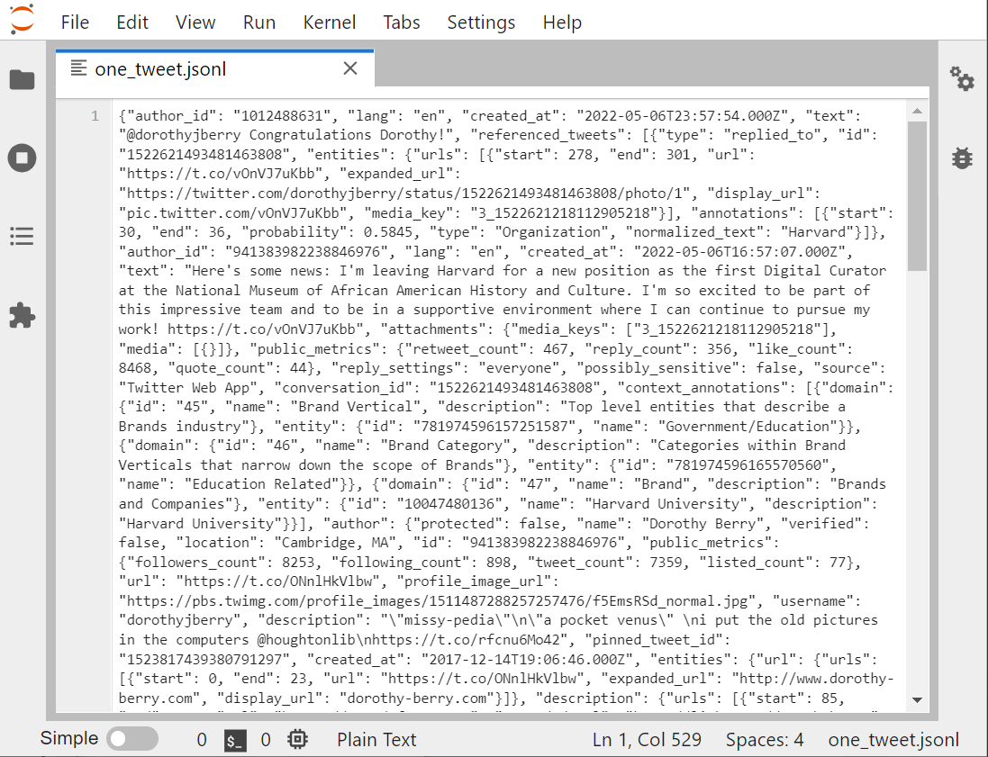
Let’s look at one individual tweet file, in the Jupyter viewer.

There are several other ways to look at any text file in the Jupyter environment: 1 Run the cat Bash command. That’s not so readable 1 Open the file with the nano editor: nano opens files unwrapped, so you can see the lines. 1 Jupyter text viewer/editor

The Jupyter viewer/editor has numbering, so we can see that this whole screen is one line. Looking at the beginning of the file, if you insert some returns and some tables, it will help you to see that JSON is a whole bunch of named-value pairs? ie:

"name": "Joe Gaucho",
"address": "123 Del Playa",
"age": 23,
"email": "jgaucho@ucsb.edu",

You can see that the key is in quotes, then there’s a colon, then the value. If the value is text, that’s going to be in quotes too.

Both nano and the Jupyter editor allows us to format the text with returns and indents, so that the individual named-value pairs are easier to identify.

JSONL vs. JSON

• JSON and JSONLs are both data structure formats based on JavaScript syntax.
• JSONLs consist of separate JSON objects in each line. A JSON object refers to an individual set or unit of data in the JSON format.
• JSONLs are more efficient to read than JSON file and are better at containing ‘objects of data’.

In our case, a single tweet acts as a single JSON object and the JSONL acts as the file that stores all of them. JSONLs better for collecting twitter data, since JSON’s are not as effective at storing multiple units of data in comparison.

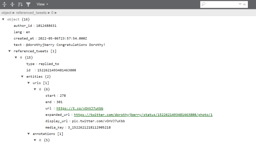
Just to show you the the contents of a single tweet, look to the output below. The output is an edit of the data with only white-space characters. These edits have been made to explore and separate the tweet’s content from the metadata.

We can see that the 4th piece of data in the tweet is “text”, and is after the author’s ID, the language, and time stamp. The fifth element, “referenced tweet”, tells us that this tweet is in reply to another tweet.

{"data": [{"author_id": "1012488631",
"lang": "en",
"created_at": "2022-05-06T23:57:54.00Z",
"text": "@dorothyjberry Congratulations Dorothy!",
"referenced_tweets": [{"type": "replied_to",
                       "id": "1522621493481463808"}],
"entities":
    {"mentions":
        [{"start": 0,
          "end": 14,
          "username": "dorothyjberry",
          "id" : "941383982238846976"}],
     "annotations": [{"start": 31, "end": 37,
          "probability": 0.8784,
          "type": "Person", "normalized_text": "Dorothy"}]},
     "in_reply_to_user_id": "941383982238846976"
     "public_metrics": {"retweet_count": 0,
           "reply_count": 0,
           "like_count": 1,
           "quote_count": 0},
reply_settings": "everyone",
"possible_sensitive": false,
"id": "1522727385380143105",
"source": "Twitter Web App",
"conversation_id": "1522621493481463808"},

There are many, many elements attached to each Tweet. You will probably never use most of them.

Some key pieces of a Tweet are:

• created_at: the exact day and time (in GMT) the tweet was posted
• id: a unique tweet ID number
• entities: strings pulled out of a tweet that line up with Twitter’s ontology
  • any hashtags that are used
  • any users who are @’ed
  • personal names

• referenced_tweets.retweeted.id’ if this is a retweet, this field shows the id of the original tweet.

• user
  • id
  • name
  • screen name (twitter handle)
  • followers_count (at the time the tweet was created)

All of these elements become much more visible if we download our tweet and open it up with an online JSONL viewer

We can also see just the name of each field by using the columns method on any dataframe we have made from Twitter data. For example, ecodatasci_df, the dataframe created from the ecodatasci timeline:

list(bjules_df.columns)

['id',
 'conversation_id',
 'referenced_tweets.replied_to.id',
 'referenced_tweets.retweeted.id',
 'referenced_tweets.quoted.id',
 'author_id',
 'in_reply_to_user_id',
 'retweeted_user_id',
...
 '__twarc.retrieved_at',
 '__twarc.url',
 '__twarc.version',
 'Unnamed: 73']

This gives you a sense of just how much data comes along with a tweet. The final three entries are added by the Twitter API to let you know how the tweet was retrieved.

First and last tweets

Let’s look at our bjules_flat.jsonl file again.

Remember our JSONL files are line-oriented, ie: one tweet per line. Let’s use the head and tail command to create files with the first and last lines of our data file.

The double-greater-than >> appends rather than creates.

!head -n 2 'output/bjules_flat.jsonl' > 'output/2_tweets.jsonl'

!tail -n 2 'output/bjules_flat.jsonl' >> 'output/2_tweets.jsonl'

If we use ! cat to output the files, we see a real mess. Let’s open the Jupyter graphical file viewer instead.

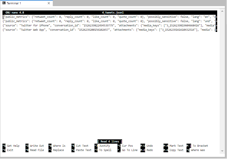
Why not use nano?

Nano, which we can call from the shell window, is a great way to stay in our little shell window with our hands on our keyboards. However, we are going to spend our workshop in Jupyter to make our work more reproducible.

However, sometimes it’s going to be advantageous to look at a file in nano, because the JSONL files open with lines unwrapped. Our 2-tweets file, for example

Using either method, it’s still difficult to tell what’s going on. Can we even tell where one tweet ends, and the second begins? Jupyter does have line numbers, so at least we can see it’s 2 lines.

With the lines unwrapped, you can advance across the line to see the posted date of the action on the timeline, as well as what type of action it was.

With the first and last tweets, that gives us the the date and time range of what we retrieved from Mr. Jules’ timeline:

#FIXME you need a new 2-tweet version

A Very Basic Analysis

One goal for us is to look at our data without looking at the JSONL directly. When we harvest tweets, it is a very good idea to do a little exploratory, reality-checking, analysis to make sure you got what you expected. As we did in the previous episode, let’s look at the bash command wc (word count) to see how many lines of JSONL, therefore how many tweets, are in our gas prices file. Don’t forget to flatten it first!

! twarc2 flatten raw/hashtag_gas.jsonl output/hashtag_gas_flat.jsonl
! wc output/hashtag_gas_flat.jsonl

15698   7653538 100048736 hashtag_gas_flat.jsonl

We can then look at the timestamps of the first and last tweets to determine the date range of our tweets by using the head and tail commands to get the first line and last line of the file:

!head -n 1 'output/hashtag_gas_flat.jsonl'
!tail -n 1 'output/hashtag_gas_flat.jsonl'

Lets save this output into a file named “gas_date_range.jsonl”:

!head -n 1 'output/hashtag_gasprices_flat.jsonl' > 'output/gasprice_range.jsonl'
!tail -n 1 'raw/hashtag_gasprices_flat.jsonl' >> 'output/gasprice_range.jsonl'

#FIXME : let’s make objects or files for these that have the date ranges pulled out.

Let’s go back and do this basic analysis for our two other files of raw data: bjules.jsonl and ecodatasci.jsonl (or whatever timeline you downloaded in the episode 2 challenge).

Challenge: Getting Date Ranges

Please create the files bjules_range.jsonl and ecodatasci_range.jsonl that contains the first and last tweets of bjules.jsonl and ecodatasci.jsonl. Use one notebook cell per file.

Remember to specify where to store your output files.

Output your answers in your notebook by creating objects and outputting them to an output cell using #FIXME …

1. What are the oldest and newest items on Bergis’ timeline.
2. How many items are on Bergis’ timeline?
3. Same questions for the timeline you downloaded in episode 2.

Solution

#FIXME this solution is not correct. the input file is wrong.

!head -n 1 'raw/bjules.jsonl' > 'output/bjules_range.jsonl'
!tail -n 1 'raw/bjules.jsonl' >> 'output/bjules_range.jsonl'
!wc 'raw/bjules.jsonl'

We can see that we retrieved Bergis’ texts back to 2018.

!head -n 1 'raw/ecodatasci.jsonl' > 'output/ecodatasci_range.jsonl'
!tail -n 1 'raw/ecodatasci.jsonl' >> 'output/ecodatasci_range.jsonl'
!wc 'raw/ecodatasci.jsonl'

Other things we can do: sentiment analysis (FORESHADOWING). See when he joined Twitter (hint: way before 2018)

Why we flatten our twarc JSONL file

In our case, a raw or unflattened JSONL will consist of lines of API requests containing multiple tweets. Therefore, we want to flatten our JSONL file in order to isolate these tweets and ensure that each line in our JSONL file consists of a single tweet instead of a single API request.

How are the flattened and unflattened versions different?

The property “Flat” refers to the structure of JSON or JSONL files. A JSON is not flat when it has a nested structure. A nested structure occurs when data consists of an attribute or attributes that contain other attributes. Flattening isolates our desired attributes so that the data can be read linearly and separately.
Here’s a rough illustration of the differences between flattend and unflattend twitter data:

Unflattened twitter data:

{"data": [{"author_id": "1", "public_metrics": {"retweet_count": 0, "reply_count": 0, "like_count": 0, "quote_count": 0}
      ... {"author_id": "2", "public_metrics": {"retweet_count": 18, "reply_count": 1, "like_count": 10, "quote_count": 2}
      ... {"author_id": "3", "public_metrics": ... ]}

Flattened twitter data:

1 {"author_id": "1", "public_metrics": {"retweet_count": 0, "reply_count": 0, "like_count": 0, "quote_count": 0} ... }
2 {"author_id": "2", "public_metrics": {"retweet_count": 18,"reply_count": 1, "like_count": 1, "quote_count": 2} ... }
3 {"author_id": "3", "public_metrics": ... }
... 

Because twarc timeline outputs API requests instead of individual tweets we need flatten or csv.

Challenge: First and last Tweets

Using the terminal or Jupyter, use the commands head and tail to save more than just the first 2 and last 2 tweets in hashtag_gasprices.jsonl. let’s say the first and last 10. View the file to determine:

1. How long is the time difference between the first and the last tweets?
2. Judging by these 20 tweets, do they arrive in chronological order?
3. Create a dataframe of these 20 tweets to look at the times in a more friendly way.

!head -n 10 'output/hashtag_gas_flat.jsonl' >  'output/20tweets.jsonl'
!tail -n 10 'output/hashtag_gas_flat.jsonl' >> 'output/20tweets.jsonl'

Solution

1. First Tweet in the file arrived Mon Apr 18 21:59:14, Final Tweet at Mon Apr 18 18:15:33. So these are Tweets span about 4 hours.
2. Answer: They arrive in reverse-chronological, with the most recent Tweets are on top, oldest at the bottom.

   {"created_at": "Mon Apr 18 21:59:14 +0000 2022", "id": 1516174539742494723, ...
   {"created_at": "Mon Apr 18 21:59:12 +0000 2022", "id": 1516174533732016132, ...
   {"created_at": "Mon Apr 18 18:15:33 +0000 2022", "id": 1516118249443844102, ...
   {"created_at": "Mon Apr 18 18:15:33 +0000 2022", "id": 1516118248110100483, ...
   

Well? Can we scroll through and examine it?

Key Points

• Tweets arrive as JSONL, a super common format.

• We can use online viewers for a human-readable look at JSONL

• Tweets come with a TON of associated data