Introduction to Topological Data Analysis

Overview

Teaching: 25 min
Exercises: 25 min

Questions

What is topological data analysis?

Objectives

Understand that simplices comprise vertices, edges, triangles, and higher dimensions structures.

Topological data analysis

Topological data analysis (TDA) is a technique that uses concepts from topology to analyze complex data and find patterns and structures that are not apparent at first glance. This technique is based on constructing a simplicial complex composed of a collection of simple geometric objects called simplices. The topology of this complex is used to analyze and visualize the relationships between the data.

Simplex

A simplex (plural simplices) is a simple geometric object of any dimension (point, line segment, triangle, tetrahedron, etc.). Simplices are used to construct simplicial complexes. The following figure shows some examples of simplices.

Simplex

Mathematical definition

Given a set $ P=\{p_0,…,p_k\}\subset \mathbb{R}^d $ of $ k+1 $ affinely independent points, the k-dimensional simplex $\sigma$ (or k-simplex for short) spanned by $P$ is the set of convex combinatios

$ \sum_{i=0}^k\lambda_ip_i, \quad with \quad \sum_{i=0}^k\lambda_i = 1 \quad \lambda_i \geq 0. $

The points $p_0, …, p_k$ are called the vertices of $\sigma$.

Simplicial complex

A simplicial complex is a mathematical structure comprising a collection of simplices constructed from a data set. In other words, a simplicial complex is a collection of vertices, edges, triangles, tetrahedra, and other elements that follow specific rules. As a starting point, we can think of a simplicial complex as extending the notion of a graph only formed by vertices and edges. The following figure shows an example of a simplicial complex.

Simplicial complex

Mathematical definition

A simplicial complex $K$ in $ \mathbb{R}^d $ is a collection of simplices s.t:

Any face of a simplex from $K$ is also a simplex of $K$,

The intersection of any two simplices of $K$ is either empty or a common face of both«.

More generally, we can define a simplicial complex as:
Let $P= \{p_1,…,p_n\}$ be a (finite) set. An abstract simplicial complex $K$ with vertex set $P$ is a set of subsets of $P$ satisfying the two conditions:

the elements of $P$ belong to $K$,

if $\tau \in K$ and $\sigma \subset \tau$, then $\sigma \in K$.

The elements of $K$ are the simplices.

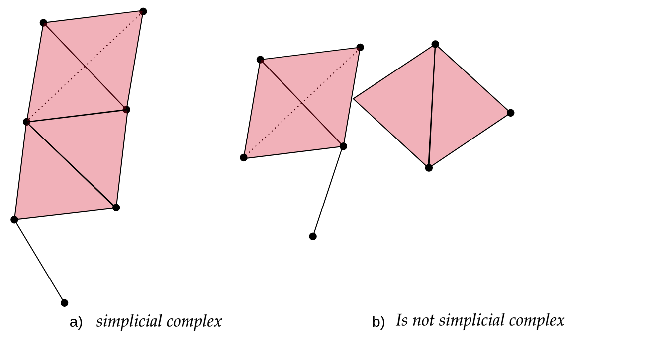
In the following figure, the left panel “a)” is an example of a simplicial complex, while the right panel “b)” is not because it does not satisfy the second mathematical condition. In the figure, a triangle is part of the simplicial complex but one vertex is not. Colloquially speaking it fails that if one simplex is part of the simplicial complex, then all its simplices of the lower dimensions must also be part of the complex. Mathematically speaking, it is not true that the face of a simplex from $K$ is also a simplex of $K$ or that the intersection of any pair of simplices is either empty or a face.

Simplicial complexes can be seen simultaneously as geometric/topological spaces (suitable for topological/geometrical inference) and as combinatorial objects (abstract simplicial complexes, suitable for computations).

Exercise 1(Beginner): Identify the simplices

In the following graph, we have two representations of simplicial complexes.

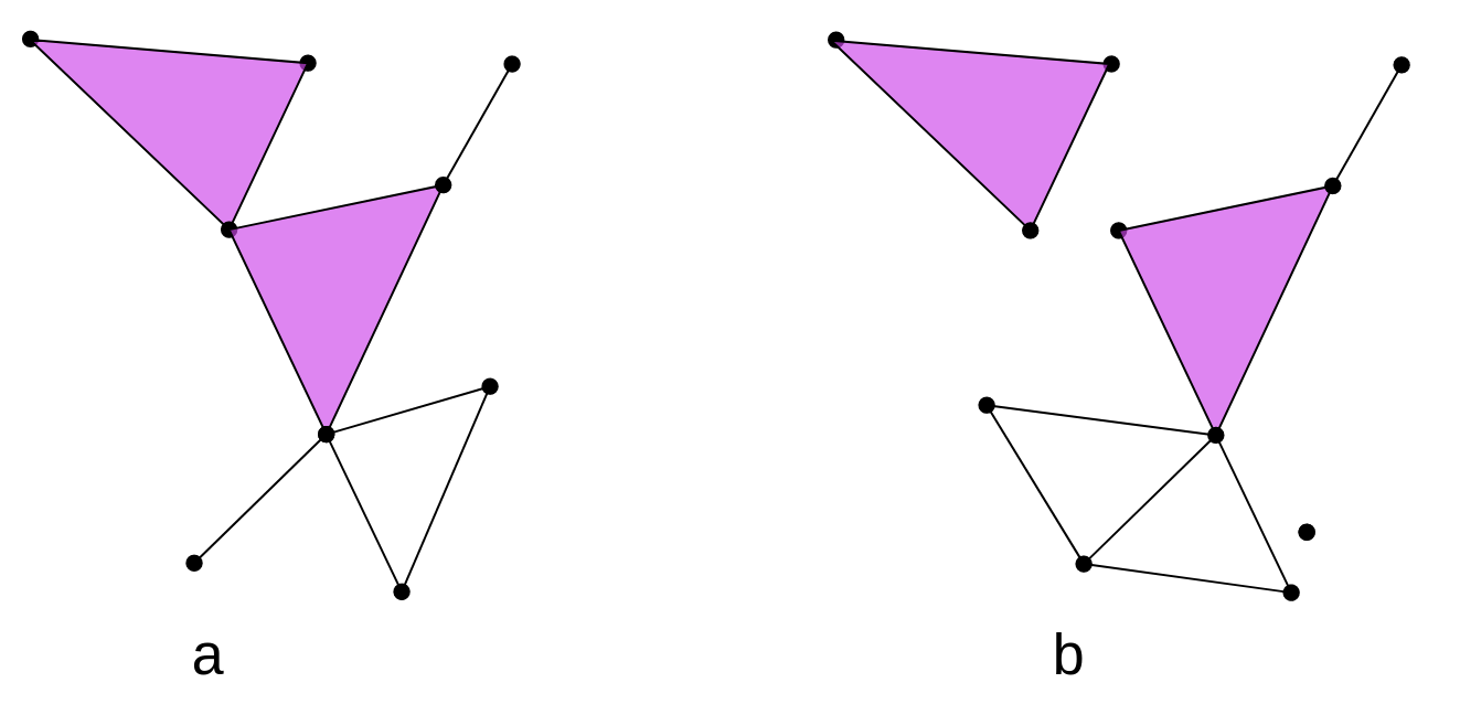
In this figure, How many 0-simplices(vertices), 1-simplices(edges), and 2-simplices(triangles) does each one of the simplicial complexes have?

Solution

Figure a Figure b

$0-simplex$ 9 11

$1-simplex$ 11 12

$2-simplex$ 2 2

	Figure a	Figure b
$0-simplex$	9	11
$1-simplex$	11	12
$2-simplex$	2	2

Čech and (Vietoris)-Rips complexes

Vietoris-Rips complex and Čech complex are two types of simplicial complexes constructing discrete structures from sets of points in space.

The Vietoris-Rips complex is constructed from a set of points in a metric space. Given a set of points and a distance parameter called the “threshold,” points within a distance less than or equal to the threshold are connected, forming the 1-simplices of the complex. Higher-dimensional simplices are then constructed by closing under combinations of 1-simplices that form a complete simplex, i.e., all fully connected subsets. The Vietoris-Rips complex captures the connectivity information between points and their topological structure at different scales.

In a practical example, the set of points represents your dataset, such as a group of genomes, and the distance could be a Hamming distance. ‘Threshold’ represents the selected distance at which two genomes are considered to be related.

Vietoris complex

Mathematical definition

Given a point cloud $P=\{p_1,…,p_n\}\subset \mathbb{R}^d $, its Rips complex of radius $r>0$ is the simplicial complex $R(P,r)$ such that:
$vert(R(P,r))=P$, and
$\sigma = [p_{i_0},p_{i_1},...,p_{i_k}] \in R(P,r) \quad iff \quad \lVert p_{i_j} -p_{i_l} \rVert \leq 2r, \forall j,l\leq k$ with $j \neq k$

On the other hand, the Čech complex is based on constructing simplicial cells rather than simply connecting points at specific distances. Given a set of points and a distance parameter, all sets of points whose balls of radius equal to the distance parameter have a non-empty intersection are considered. These sets of points become the simplices of the Čech complex. Similar to the Vietoris-Rips complex, higher-dimensional simplices can be constructed by closing under combinations of lower-dimensional simplices that form a complete simplex.

Čech complex

Mathematical definition

Given a point cloud $P=\{p_1,…,p_n\}\subset \mathbb{R}^d$, its Cech complex of radius $r>0$ is the simplicial complex $C(P,r)$ such that: $vert(C(P,r))=P$, and
$\sigma = [p_{i_0},p_{i_1},...,p_{i_k}] \in C(P,r) \quad iff \quad \cap_{j=0}^k Bp_{i_j} \neq \emptyset$

In the following figure, we have the representation of the Rips simplicial complex (left) and the Cech simplicial complex (right), for the same set of points $P={p_1,…,p_9}$.

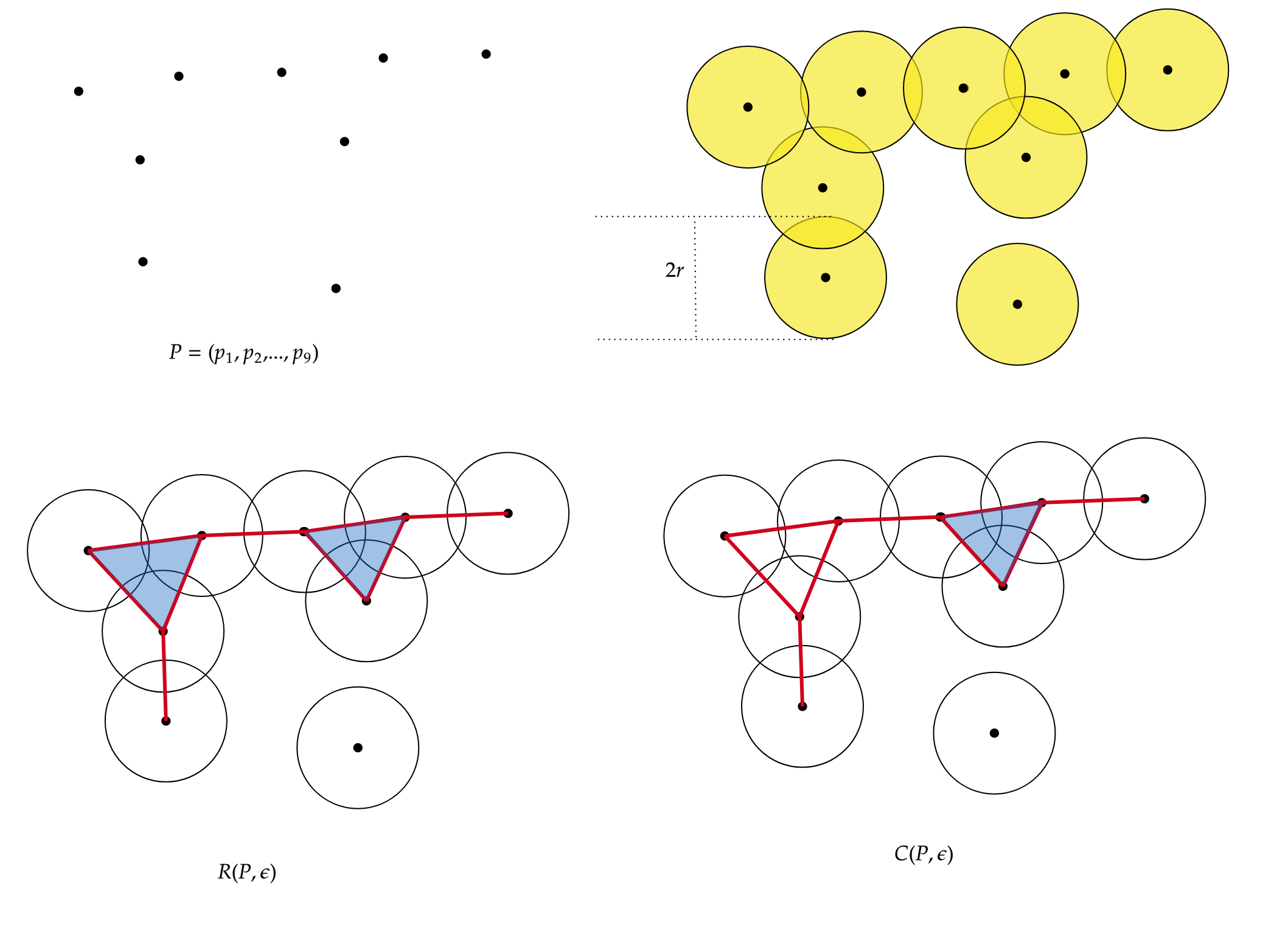
The following table shows the number of simplices for each simplicial complex.

	$R(P,r)$	$C(P,r)$
$0-simplex$	9	9
$1-simplex$	9	9
$2-simplex$	2	1

The difference lies in the $2-simplices$. Given 3 points, to construct a 2-simplex (triangle) in the Cech complex, the 3 balls of radius $r$ must intersect each other, while in the Rips complex, the balls must intersect pairwise.”

Both the Vietoris-Rips complex and the Čech complex are tools used in topological analysis and computational geometry to study the structure and properties of sets of points in space. These complexes provide a discrete representation of the proximity and connectivity information of the points, enabling the analysis of their topology and geometric characteristics.

Note

Čech complexes can be quite hard to compute.

Simplicial homology

Simplicial homology is a technique used to quantify the topological structure of a simplicial complex. This technique is based on identifying cycles and voids in the complex, which can be quantified by assigning integer values called “homology degrees”. Simplicial homology is often used in topological data analysis to find patterns and structures in the data. Some definitions that we must keep in mind are the following.

Holes: Holes are empty regions or connected spaces in a simplicial complex. Simplicial homology allows for the detection and quantification of the presence of holes in the complex.

Connected Components: Connected components are sets of simplices in a simplicial complex that are connected to each other through shared simplices. Simplicial homology can identify and count the connected components in the complex.

Betti Numbers: Betti numbers are numerical invariants that measure the number of connected components and holes in a simplicial complex. Betti-0 ($\beta_0$) counts the number of connected components, while Betti-1 ($\beta_1$) counts the number of one-dimensional holes.

Exercise 2(Beginner): Identify Betti numbers

In the following graph, we have 2 representations of simplicial complexes.

What are the $\beta_0$ and $\beta_1$ of these simplicial complexes in the image?.

Hint: Remember that a painted triangle (color rose in this case) represents a 2-simplex, while an uncolored triangle represents a missing triangle that forms a 1-hole.

Solution

Figure A Figure B

$\beta_0$ 1 3

$\beta_1$ 1 2

	Figure A	Figure B
$\beta_0$	1	3
$\beta_1$	1	2

Filtration

A filtration of a simplicial complex is an ordered sequence of subcomplexes of the original complex, where each subcomplex contains its predecessor in the sequence. In other words, it is a way to decompose the complex into successive stages, where each stage adds or removes simplices compared to the previous stage.

Filtration

Mathematical definition

A filtration of a simplicial complex $K$ is a collection $K_0\subset K_1 \subset …\subset K_N $ of complexes satisfying the two conditions:

$K_N=K$.

$K_i$ is a subcomplex of $K_{i+1}$, for $i=0,1,…,N-1$.

An example of a filtration for $K=\langle a, b , c \rangle $ is the following:

In this case, we have 5 levels of filtration. The red color represents the simplices that are being added at each level of filtration, starting from $K_0$ with the vertices ${a,b,c}$ and ending at $K_4=\langle a, b, c \rangle $, the triangle (including the face) with vertices $a,b,c$.

Now, to apply persistent homology, we need to vary the parameters associated with the filtration. In the filtration graph, we have 5 distinct steps for the filtered simplicial complex. In each of these steps, we can have a different number of connected components and 1-holes.

Exercise 3(Intermediate): Calculate the Betti numbers.

For the filtration shown in Figure 1, calculate the Betti numbers ($\beta_0 $ and $\beta_1$)for each level of the filtration

Solution

$\beta_0$ $\beta_1$

$K_0$ 3 0

$K_1$ 2 0

$K_2$ 1 0

$K_3$ 1 1

$K_4$ 1 0

	$\beta_0$	$\beta_1$
$K_0$	3	0
$K_1$	2	0
$K_2$	1	0
$K_3$	1	1
$K_4$	1	0

We can observe that at the beginning (filtration level 0), we have 3 connected components. At filtration level 1, we have 2 connected components, meaning that 2 connected components merged to form a single one, or we can also say that one connected component died. The same thing happens at filtration level 2, leaving us with only one connected component. At filtration level 3, we still have one connected component, but a 1-hole appears. Finally, at filtration level 4, we still have one connected component, and the 1-hole disappears.

To visualize these changes, we will use a representation with the following persistence diagrams and barcode.

Persistence Diagram

The persistence diagram is a visual representation of the evolution of cycles and cavities in different dimensions as the simplicial complex is modified. It helps understand the persistence and relevance of topological structures in the complex.

Continuing with the example of the filtration of $K$, to construct the persistence diagram, we need to empty the information we obtained in the previous exercise.

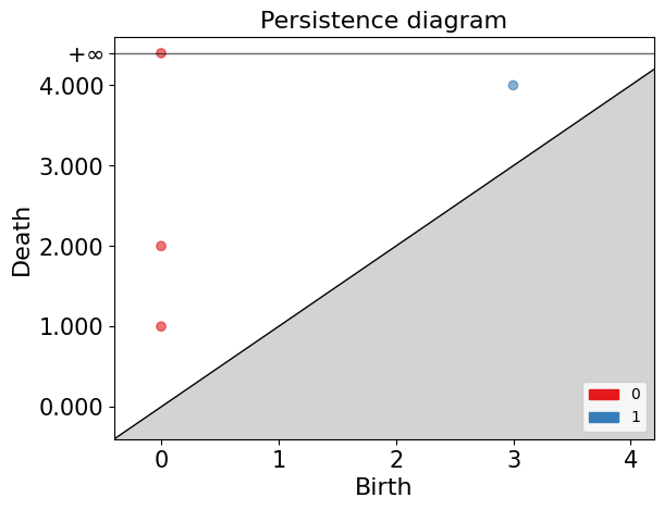
In the persistence diagram, connected components are represented in red, and 1-holes are shown in blue. The $x$ and $y$ axes represent the filtration levels and are labeled as “birth” and “death” respectively. The coordinates of the points indicate when each connected component or 1-hole was born and died. Additionally, there is a connected component that has infinite death time, meaning it never dies during filtration. This is referred to as “infinite persistence”.

Barcode Diagram

A barcode diagram is a graphical tool used to visualize the persistence diagram. It consists of bars representing the persistence intervals of cycles and cavities, indicating their duration and relevance in the simplicial complex.

In the barcode diagram, the $X$ axis represents the filtration levels, and the beginning of a red bar indicates the birth of a connected component, while the end of that bar represents its death (i.e., when it merged with another component). For the blue bars, the idea is analogous, but they represent 1-holes instead.

App to play

This app, created in GeoGebra by José María Ibarra Rodríguez (jose.ibarra@c3consensus.com), allows us to manipulate the parameter $r$ to construct a Rips simplicial complex for a set of 16 points in $\mathbb{R}^2$. Additionally, it enables us to view the barcode of the filtration and visualize the simplices as they are formed.

Steps to use:

Click on the square button in the bottom right corner to maximize the app.
In the top right corner, there is a slider for the values of $r$ that you can adjust according to your preferences.
At the bottom, you can select what you want to display, such as simplices, balls, and the barcode.

Exercise 4(Advanced): Using the app example

Using the application, answer the following questions:

a. For what value of $r$ does the 1-simplex (edge) appear?
b. For what value of $r$ do we have only one connected component ($\beta_0 = 1$)?
c. How many 1-holes appear, and for what values of $r$ do they appear?
d. Persistence is defined as the difference between birth and death. What is the persistence of the 1-holes?
e. What can that persistence tell us about the shape of the data?

Solution

a. $r=0.5$
b. $r=0.83$
c. Two. The first one $r=0.76$ and the second one $r=0.86$.
d. The persistence is $0.12$ and $1.65$.
e. The second hole has a significant persistence of $1.6$, which suggests that the data is indeed arranged in a circular manner.

Key Points

TDA describes data forms.

Betti numbers allows us to find conected components and 1-holes in data sets.

Computational Tools for TDA

Overview

Teaching: 30 min
Exercises: 15 min

Questions

How can I computationally manipulate simplicial complexes?

Objectives

Operate simplicial complexes in a computational environment

Create Vietoris-Rips and Alpha complexes from diverse datasets

Apply persistent homology to obtain barcode and persistence diagrams

Introduction to GUDHI and Simplicial Homology

Welcome to this lesson on using GUDHI and exploring simplicial homology. GUDHI (Geometry Understanding in Higher Dimensions) is an open-source that provides algorithms and data structures for the analysis of geometric data. It offers a wide range of tools for topological data analysis, including simplicial complexes and computations of their homology.

To begin, we will import the necessary packages.

from IPython.display import Image     # Import the Image function from IPython.display to display images in Jupyter environments.
from os import chdir                  # Import chdir from os module to change the current working directory.
import numpy as np                    # Import numpy library for working with n-dimensional arrays and mathematical operations.
import gudhi as gd                    # Import gudhi library for computational topology and computational geometry.
import matplotlib.pyplot as plt       # Import pyplot from matplotlib for creating visualizations and graphs.
import argparse                       # Import argparse, a standard library for writing user-friendly command-line interfaces.
import seaborn as sns                 # Import seaborn for data visualization; it's based on matplotlib and provides a high-level interface for drawing statistical graphs.
import requests                       # Import requests library to make HTTP requests in Python easily.

Example 1: SimplexTree and Manual Filtration

The SimplexTree data structure in GUDHI allows efficient manipulation of simplicial complexes. You can demonstrate its usage by creating a SimplexTree object, adding simplices manually, and then filtering the complex based on a filtration value.

Create SimplexTree

With the following command, you can create a SimplexTree object named st, which we will use to add the information of your filtered simplicial complex:

st = gd.SimplexTree()  ## 

Insert simplex

In GUDHI, you can use the st.insert() function to add simplices to a SimplexTree data structure. Additionally, you have the flexibility to specify the filtration level of each simplex. If no filtration level is specified, it is assumed to be added at filtration time 0.

#insert 0-simplex (the vertex) 
st.insert([0])
st.insert([1])

True

Now let’s insert 1-simplices at different filtration levels. If adding a simplex requires a lower-dimensional simplex to be present, the missing simplices will be automatically completed.

Here’s an example of inserting 1-simplices into the SimplexTree at various filtration levels:

# Insert 1-simplices at different filtration levels
st.insert([0, 1], filtration=0.5)
st.insert([1, 2], filtration=0.8)
st.insert([0, 2], filtration=1.2)

True

Note

If any lower-dimensional simplices are missing, GUDHI’s SimplexTree will automatically complete them. For example, when inserting the 1-simplex [1, 2] at filtration level 0.8, if the 0-simplex [1] or [2] was not already present, GUDHI will add it to the SimplexTree.

Now, you can use the st.num_vertices() and st.num_simplices() commands to see the number of vertices and simplices, respectively, in your simplicial complex stored in the st SimplexTree object.

num_vertices = st.num_vertices()
num_simplices = st.num_simplices()

print("Number of vertices:", num_vertices)
print("Number of simplices:", num_simplices)

Number of vertices: 3
Number of simplices: 6

Persistence

The st.persistence() function in GUDHI’s SimplexTree is used to compute the persistence diagram of the simplicial complex. The persistence diagram provides a compact representation of the birth and death of topological features as the filtration parameter varies.

Here’s an example of how to use st.persistence():

# Compute the persistence diagram
persistence_diagram = st.persistence()

# Print the persistence diagram
for point in persistence_diagram:
    birth = point[0]
    death = point[1]
    print("Birth:", birth)
    print("Death:", death)
    print()

Birth: 0
Death: (0.0, inf)

Birth: 0
Death: (0.0, 0.5)

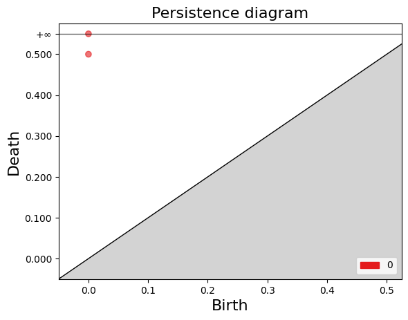
Plot the persistence diagram

The gd.plot_persistence_diagram(persistence_diagram, legend=True) is used to plot a persistence diagram using the Gudhi library in Python. A persistence diagram is a visual representation of the topological features captured by the simplicial homology computation.

The plot_persistence_diagram() function takes the persistence diagram as input and generates a plot to visualize this information. The legend=True argument enables the display of a legend, which provides additional information about the different types of topological features represented in the diagram.

gd.plot_persistence_diagram(persistence_diagram,legend=True)

<AxesSubplot:title={'center':'Persistence diagram'}, xlabel='Birth', ylabel='Death'>

Plot the barcode

The code snippet gd.plot_persistence_barcode(persistence_diagram, legend=True) is used to generate a persistence barcode plot using the Gudhi library in Python. A persistence barcode provides a different way to visualize the evolution of topological features captured by the persistence diagram.

In topological data analysis, a persistence barcode represents the lifespan of topological features as intervals on a real number line. Each interval corresponds to a topological feature, and its length represents the duration of the feature’s existence.

The plot_persistence_barcode() function takes the persistence diagram as input and generates a plot that visualizes these intervals. The bars in the barcode plot represent the topological features, and their lengths indicate the duration of their existence.

gd.plot_persistence_barcode(persistence_diagram,legend=True)

<AxesSubplot:title={'center':'Persistence barcode'}>

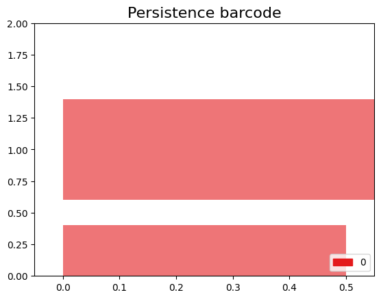
By examining the persistence barcode plot, one can observe the distribution and lengths of the bars. Longer bars indicate more persistent topological features, while shorter bars represent features that appear and disappear quickly. The legend displayed with legend=True provides additional information about the types of topological features represented in the barcode.

This visualization allows for the identification of significant topological features and their persistence across different scales. It provides insights into the robustness and stability of these features in the dataset, helping to reveal important structural patterns and understand the underlying topology of the data.

Exercise 1(Intermediate): Creating a Manually Filtered Simplicial Complex.

In the following graph, we have $K$ a simplicial complex filtered representation of simplicial complexes. Perform persistent homology and plot the persistence diagram and barcode.
Solution

Step 1: Create a SimplexTree with gd.SimplexTree().
st = gd.SimplexTree()  
Step 2: Insert vertices at time 0 using st.insert()
#insert 0-simplex (the vertex), 
st.insert([0])
 st.insert([1])
st.insert([2])
 st.insert([3])
 st.insert([4])
Step 3: Insert the remaining simplices by setting the filtration time using st.insert([0, 1], filtration=).
#insert 1-simplex level filtration 1 
st.insert([0, 2], filtration=1)
st.insert([3, 4], filtration=1)
#insert 1-simplex level filtration 2 
st.insert([0, 1], filtration=2)
#insert 1-simplex level filtration 3 
 st.insert([2, 1], filtration=3)
#insert 1-simplex level filtration 4 
st.insert([2, 1,0], filtration=4)
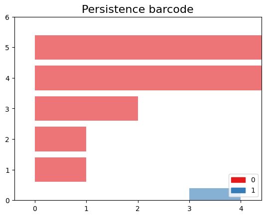
Step 4: Perform persistent homology using st.persistence().
# Compute the persistence diagram
persistence_diagram = st.persistence() 
Step 5: Plot the persistence diagram.
# plot the persistence diagram
gd.plot_persistence_diagram(persistence_diagram,legend=True)
Step 6: Plot the barcode.
gd.plot_persistence_barcode(persistence_diagram,legend=True)
Step 7: Get this output

Example 2: Rips complex from datasets

In this example, we will demonstrate an application of persistent homology using a dataset generated by us. Persistent homology is a technique used in topological data analysis to study the shape and structure of datasets.

Generate dataset

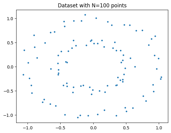
The make_circles() function from scikit-learn’s datasets module is used to generate synthetic circular data. We specify the number of points to generate (n_samples), the amount of noise to add to the data points (noise), and the scale factor between the inner and outer circle (factor).

The generated dataset consists of two arrays: circles and labels. The circles array contains the coordinates of the generated data points, while the labels array assigns a label to each data point (in this case, it will be 0 or 1 representing the two circles).

from sklearn import datasets  # Import the datasets module from scikit-learn

# Generate synthetic data using the make_circles function
# n_samples: Number of points to generate
# noise: Standard deviation of Gaussian noise added to the data
# factor: Scale factor between inner and outer circle
circles, labels = datasets.make_circles(n_samples=100, noise=0.06, factor=0.5)

# Print the dimensions of the generated data
print('Data dimension: {}'.format(circles.shape))

Data dimension:(100, 2)

Plot dataset

fig = plt.figure()  # Create a new figure
ax = fig.add_subplot(111)  # Add a subplot to the figure
ax = sns.scatterplot(x=circles[:,0], y=circles[:,1], s=15)  # Create a scatter plot using seaborn
plt.title('Dataset with N=%s points'%(circles.shape[0]))  # Set the title of the plot
plt.show()  # Display the plot

Create Rips complex

First, we create a Rips complex using the RipsComplex class from gudhi. The Rips complex is a simplicial complex constructed from the given data points by connecting them with edges if their pairwise distances are below a specified threshold. In this case, we set the max_edge_length parameter to 0.6, which determines the maximum length allowed for an edge to be included in the complex.

%%time
# Create a Rips complex with a maximum edge length of 0.6
Rips_complex = gd.RipsComplex(points = circles, max_edge_length=0.6)

CPU times: user 461 µs, sys: 88 µs, total: 549 µs
Wall time: 557 µs

Next, we create a simplex tree using the create_simplex_tree() method of the Rips_complex object. The simplex tree is a data structure that stores the information about the simplices in the complex. We specify max_dimension=3 to include simplices up to dimension 3 in the complex.

%%time
#Create a simplex tree from the Rips complex with a maximum dimension of 3
Rips_simplex_tree = Rips_complex.create_simplex_tree(max_dimension=3) 

CPU times: user 2.25 ms, sys: 0 ns, total: 2.25 ms
Wall time: 1.95 ms

Then, we retrieve the filtration order of simplices from the Rips_simplex_tree using the get_filtration() method. Filtration is a sequence of simplices ordered by their inclusion in the complex. We convert the filtration to a list using list().

%%time
# Get the filtration order of simplices
filt_Rips = list(Rips_simplex_tree.get_filtration())

CPU times: user 108 ms, sys: 0 ns, total: 108 ms
Wall time: 121 ms

Simplicial homology

Finally, we compute the persistence of the Rips complex using the persistence() method of the Rips_simplex_tree. Persistence computes the birth and death values for each topological feature (connected components, loops, voids, etc.) in the complex. The result is assigned to the variable diag_Rips.

%%time
# Compute the persistence of the Rips complex
diag_Rips = Rips_simplex_tree.persistence()

CPU times: user 9.13 ms, sys: 41 µs, total: 9.17 ms
Wall time: 8.82 ms

Plots the persistence diagram and barcode

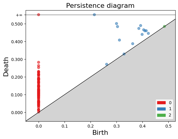
The plot_persistence_diagram() function takes the persistence diagram (diag_Rips) as input and creates a scatter plot of the points. The birth and death values are used to determine the positions of the points in the diagram.

Additionally, the legend parameter is set to True, which displays a legend in the plot. The legend provides information about the colors or markers used to differentiate different topological dimensions or features.

%%time
# Plot the persistence diagram
gd.plot_persistence_diagram(diag_Rips, legend=True)

<AxesSubplot:title={'center':'Persistence diagram'}, xlabel='Birth', ylabel='Death'>

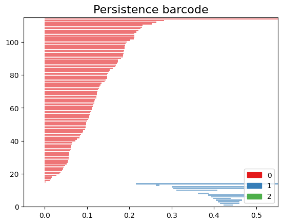
The persistence barcode is another graphical representation of the persistence pairs obtained from the computation of persistent homology. It visualizes the birth and death values of topological features as intervals on a barcode-like plot.

The plot_persistence_barcode() function takes the persistence diagram (diag_Rips) as input and creates a barcode plot. Each bar in the plot represents a topological feature, and its length corresponds to the persistence or lifetime of the feature. The x-axis represents the range of values for the birth and death of the features.

The legend parameter is set to True in order to display a legend in the plot. The legend provides information about the colors or markers used to differentiate different topological dimensions or features.

gd.plot_persistence_barcode(diag_Rips,legend=True)

<AxesSubplot:title={'center':'Persistence barcode'}>

Example 3: Rips complex from datasets

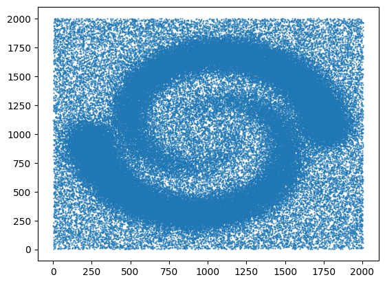
We are using the gudhi library to load a 2D point cloud data from a CSV file and visualize it using matplotlib.

First, we import the necessary modules from gudhi to work with datasets and construct the Alpha complex. We import _points from gudhi.datasets.generators to generate points and AlphaComplex to construct the Alpha complex.

from gudhi.datasets.generators import _points
from gudhi import AlphaComplex

We use the requests.get() function to send a GET request to the specified URL and retrieve the content of the file. The content is stored in the response object, and we extract the text content using response.text.

The text content is then loaded into a NumPy array using np.loadtxt(). The content.splitlines() splits the text content into lines, and delimiter=' ' specifies that the values in each line are separated by a space.

Finally, we visualize the loaded data by plotting the points using plt.scatter(). The data[:, 0] and data[:, 1] select the first and second columns of the data array, representing the x and y coordinates respectively. The marker='.' specifies the marker style as a dot, and s=1 sets the marker size. The points are then displayed using plt.show().

# Load the file spiral_2d.csv from the specified URL
url = 'https://raw.githubusercontent.com/paumayell/topological-data-analysis/gh-pages/files/spiral_2d.csv'

# Get the content of the file
response = requests.get(url)
content = response.text

# Load the data into a NumPy array
data = np.loadtxt(content.splitlines(), delimiter=' ')

# Plot the points
plt.scatter(data[:, 0], data[:, 1], marker='.', s=1)
plt.show()

we are using the AlphaComplex class from the gudhi library to construct an Alpha complex from the loaded 2D point cloud data.

First, we create an instance of the AlphaComplex class, alpha_complex, by passing the data array to the points parameter. This initializes the Alpha complex object and prepares it to construct the complex based on the given points.

Next, we create a simplex tree using the create_simplex_tree() method of the alpha_complex object. The simplex tree is a data structure that stores the information about the simplices in the Alpha complex. It represents the hierarchy of simplices in the complex, from the lowest-dimensional simplices (vertices) to higher-dimensional simplices (e.g., edges, triangles).

By calling create_simplex_tree(), we construct the simplex tree based on the Alpha complex. The simplex tree contains information about the simplices, such as their filtration values and filtration order.

The simplex_tree object can be further utilized to analyze and extract topological features and their persistence from the constructed Alpha complex. It provides various methods for computing persistence, extracting persistence diagrams, and performing other topological computations.

Overall, the code segment constructs the Alpha complex from the 2D point cloud data and creates a simplex tree to store the resulting complex’s information. This allows for subsequent topological analysis and computations on the constructed complex using the simplex_tree object.

# Construct an Alpha complex from the data points
alpha_complex = AlphaComplex(points=data)

# Create a simplex tree based on the Alpha complex
simplex_tree = alpha_complex.create_simplex_tree()

CPU times: user 5.04 s, sys: 0 ns, total: 5.04 s
Wall time: 5.06 s

diag = simplex_tree.persistence()
diag = simplex_tree.persistence(homology_coeff_field=2, min_persistence=0)
print("diag=", diag)

gd.plot_persistence_diagram(diag)

<AxesSubplot:title={'center':'Persistence diagram'}, xlabel='Birth', ylabel='Death'>

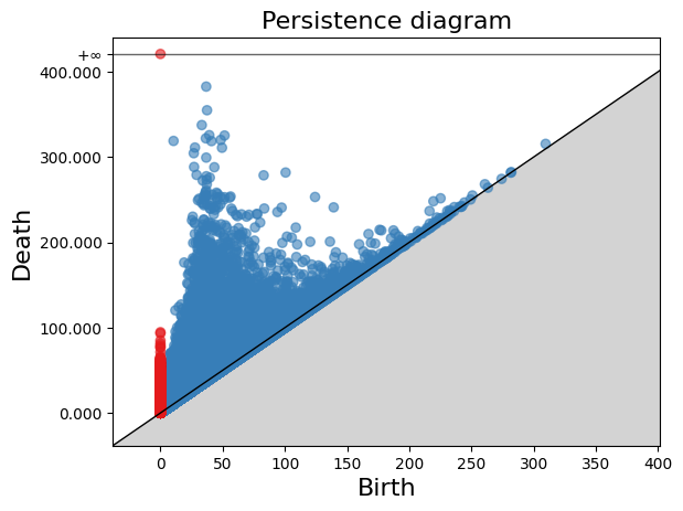
gd.plot_persistence_barcode(diag)
plt.show()

/opt/tljh/user/envs/TDA2/lib/python3.7/site-packages/gudhi/persistence_graphical_tools.py:83: UserWarning: There are 229062 intervals given as input, whereas max_intervals is set to 20000.
  % (len(persistence), max_intervals)

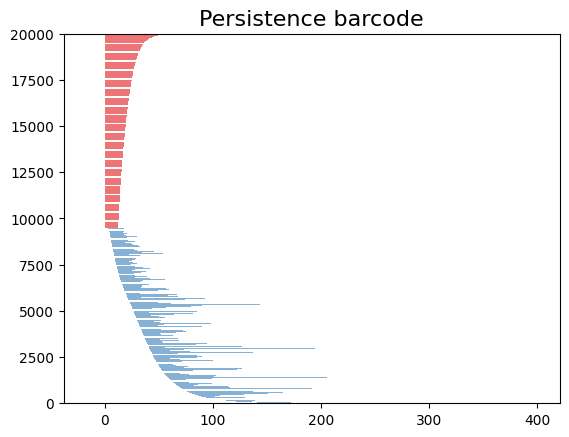
%%time
gd.plot_persistence_barcode(diag,legend=True)

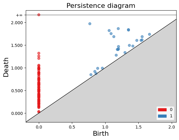
Exercise 2(Intermediate): Constructing a Torus and Analyzing Persistent Homology.

Use the tadasets.torus(n=num_points) function to generate a dataset representing a torus. Ensure that num_points is an integer specifying the number of points to generate. Once you have generated the torus, apply persistent homology techniques to analyze the topology of the dataset.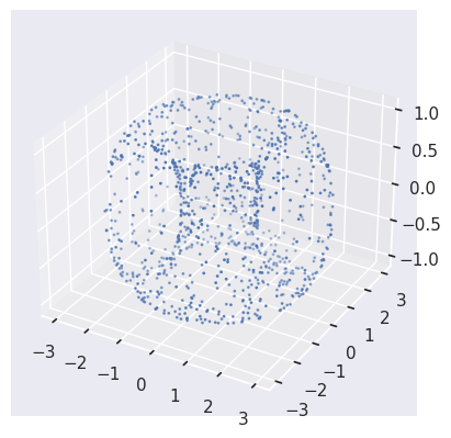
Solution
#pip install tadasets
import tadasets
import gudhi
import matplotlib.pyplot as plt
# Generate torus points
torus = tadasets.torus(n=100)
# Create a Rips complex from the torus points
rips_complex = gudhi.RipsComplex(points=torus)
# Obtain the simplicial complex
simplicial_complex = rips_complex.create_simplex_tree(max_dimension=2)
# Compute the persistent homology of the simplicial complex
persistence = simplicial_complex.persistence()
# Plot diagrams
gudhi.plot_persistence_diagram(persistence, legend=True)
plt.show()

FIXME

Add something more to the keypoints

Key Points

GUDHI is a TDA tool

GUDHI uses simplextree objects to efficiently store simplicial complexes

GUDHI allows creating simplicial complexes from datasets, distance matrices, simulated data, and manually

Detecting horizontal gene transfer

Overview

Teaching: 30 min
Exercises: 30 min

Questions

How can I detect HGT with TDA?

Objectives

Understand hierarchical data does not have 1-holes

Compute the Hamming matrix for applying Persistent Homology.

Introduction to Horizontal Gene Transfer

Horizontal gene transfer (HGT) is a process through which organisms transfer genetic material to each other in a non-traditional way without sexual reproduction. This phenomenon is particularly common among bacteria. Unlike vertical gene transfer, where genetic material is inherited from parents to offspring, HGT allows bacteria to acquire new genes directly from other organisms, potentially even from different species.

HGT is crucial in the rapid spread of antibiotic-resistant genes among bacteria, enabling them to quickly adapt to new environments and survive in the presence of antibiotics. Antibiotic resistance genes can be located on plasmids, small DNA molecules that can be easily transferred between bacteria, accelerating the spread of resistance. The horizontal transfer of antibiotic-resistance genes poses a significant challenge to global public health. It leads to the development and spread of “superbugs” resistant to multiple antibiotics, complicating the treatment of common infections and increasing mortality.

Know more: Mechanisms of HGT

Extra content

You can read more about Horizontal Gene Transfer in this Wikipedia Article. For instance, the main mechanisms of HGT are the following:

Transformation: Direct DNA uptake from the environment.

Transduction: Transfer of genes by bacteriophages (viruses that infect bacteria).

Conjugation: Transfer of genetic material between bacteria through direct contact, usually via a structure known as a pilus.

Understanding Persistent Homology in the Context of HGT:

Topological data analysis (TDA), particularly persistent homology, allows for identifying complex patterns and structures in large genomic datasets, facilitating the detection of HGT of antibiotic resistance genes. Hierarchical data does not have holes in higger dimensions when represented with a Vietoris Rips complex. A population not experiencing horizontal gene transfer and where no mutations are allowed in the same site show non-empty homology only at $ \H_0 $. Remember, $ \H_0 $ in the barcode diagram indicates the presence of connected components.

Here, we will study study cases, 1) we will show persistent homology in vertical inheritance, 2) we will study a simulation of Horizontal Gene Transfer, and 3)In the exercises, we will calculate the persistent homology of the resistant genes from Streptococcus agalactiae that we obtained in the episode Annotating Genomic Data, from the lesson Pangenome Analysis in Prokaryotes. In all three cases, we are going to need first to import some libraries, then to define functions, and finally to call them to visualize the data.

Know more: TDA in genomics

To learn more about applications of TDA in genomics, consult the Rabadan book Topological Data Analysis for Genomics

Importing Libraries

To begin, we will import the necessary packages.

import numpy as np
import pandas as pd
import seaborn as sns
import matplotlib.pyplot as plt
from scipy.cluster.hierarchy import dendrogram, linkage
import gudhi as gd
from scipy.spatial.distance import hamming

import plotly.graph_objs as go
import networkx as nx
import plotly.graph_objects as go
import plotly.io as pio

Defining Fuctions

The function calculate_hamming_matrix calculates a Hamming distance matrix from an array where the columns are genes and the rows are genomes. The hamming distance counts how many differences are in two strings. We have created several hamming distance functions in the episode functions.

# Let's assume that "population" is a numpy ndarray with your genomes as rows.
def calculate_hamming_matrix(population):
    # Number of genomes
    num_genomes = population.shape[0]
    # Create an empty matrix for Hamming distances
    hamming_matrix = np.zeros((num_genomes, num_genomes), dtype=int)
   # Calculate the Hamming distance between each pair of genomes
    for i in range(num_genomes):
        for j in range(i+1, num_genomes):  # j=i+1 to avoid calculating the same distance twice
            # The Hamming distance is multiplied by the number of genes to convert it into an absolute distance
            distance = hamming(population[i], population[j]) * len(population[i])
            hamming_matrix[i, j] = distance
            hamming_matrix[j, i] = distance  # The matrix is symmetric
    
    return hamming_matrix

The create_complex function generates a 3-dimensional Rips simplicial complex and computes persistent homology from a distance matrix.

def create_complex(distance_matrix):
    # Create the Rips simplicial complex from the distance matrix
    rips_complex = gd.RipsComplex(distance_matrix=distance_matrix)
    # Create the simplex tree from the Rips complex with a maximum dimension of 3
    simplex_tree = rips_complex.create_simplex_tree(max_dimension=3)
    # Compute the persistence of the simplicial complex
    persistence = simplex_tree.persistence()
    # Return the persistence diagram or barcode
    return persistence, simplex_tree

Function plot_dendrogram helps visualizing a cladogram.

#### Function for visualization
def plot_dendrogram(data):
    """Plot a dendrogram from the data."""
    linked = linkage(data, 'single')
    dendrogram(linked, orientation='top', distance_sort='descending')
    plt.show()

The visualize_simplicial_complex function creates a graphical representation of a simplicial complex for a given filtration level based on a simplex tree. This function is based on what you learned in the plotting episode in the lesson Introduction to Python.

def visualize_simplicial_complex(simplex_tree, filtration_value, vertex_names=None, save_filename=None, plot_size=1, dpi=600, pos=None):
    G = nx.Graph()
    triangles = []  # List to store triangles (3-nodes simplices)
    
    for simplex, filt in simplex_tree.get_filtration():
        if filt <= filtration_value:
            if len(simplex) == 2:
                G.add_edge(simplex[0], simplex[1])
            elif len(simplex) == 1:
                G.add_node(simplex[0])
            elif len(simplex) == 3:
                triangles.append(simplex)
    
    # Calculate node positions if not provided
    if pos is None:
        pos = nx.spring_layout(G)
    
    # Node trace
    x_values, y_values = zip(*[pos[node] for node in G.nodes()])
    node_labels = [vertex_names[node] if vertex_names else str(node) for node in G.nodes()]
    node_trace = go.Scatter(x=x_values, y=y_values, mode='markers+text', hoverinfo='text', marker=dict(size=14), text=node_labels, textposition='top center', textfont=dict(size=14))
    
    # Edge traces
    edge_traces = []
    for edge in G.edges():
        x0, y0 = pos[edge[0]]
        x1, y1 = pos[edge[1]]
        edge_trace = go.Scatter(x=[x0, x1, None], y=[y0, y1, None], mode='lines', line=dict(width=3, color='rgba(0,0,0,0.5)'))
        edge_traces.append(edge_trace)
    
    # Triangle traces
    triangle_traces = []
    for triangle in triangles:
        x0, y0 = pos[triangle[0]]
        x1, y1 = pos[triangle[1]]
        x2, y2 = pos[triangle[2]]
        triangle_trace = go.Scatter(x=[x0, x1, x2, x0, None], y=[y0, y1, y2, y0, None], fill='toself', mode='lines+markers', line=dict(width=2), fillcolor='rgba(255,0,0,0.2)')
        triangle_traces.append(triangle_trace)
    
    # Configure the layout of the plot
    layout = go.Layout(showlegend=False, hovermode='closest', xaxis=dict(showgrid=False, zeroline=False, tickfont=dict(size=16, family='Arial, sans-serif')), yaxis=dict(showgrid=False, zeroline=False, tickfont=dict(size=16, family='Arial, sans-serif')))
    
    fig = go.Figure(data=edge_traces + triangle_traces + [node_trace], layout=layout)
    
    # Set the figure size
    fig.update_layout(width=plot_size * dpi, height=plot_size * dpi)
    
    # Save the figure if a filename is provided
    if save_filename:
        pio.write_image(fig, save_filename, width=plot_size * dpi, height=plot_size * dpi, scale=1)
    
    # Show the figure
    fig.show()

    return G

Case Study 1: Vertical Inheritance in a Simulated Population

We simulate a bacterial population’s evolution whos inheritance is exclusively by vertical gene transfer (inheritance from parent to offspring). Applying persistent homology to this simulation, we expect a barcode diagram predominantly showing connected components ($ H_0 $), with little to no evidence of higher-dimensional features. This serves as a baseline for understanding the impact of vertical inheritance on genomic data topology.

We proceed to load a numpy array, named population_esc, which contains a resistome of a population with 8 genomes, simulated from a genome with three generations, and in each generation, one genome has 2 offspring. The total number of genes is 505, the initial percentage of 1s is 25%, and the gene gain rate in each generation is 1/505.

population_esc = np.load('https://github.com/carpentries-incubator/topological-data-analysis/raw/gh-pages/files/population_esc.npy')
population_esc

array([[0, 1, 0, ..., 0, 1, 0],
       [0, 1, 0, ..., 0, 1, 0],
       [0, 1, 0, ..., 0, 1, 0],
       ...,
       [0, 1, 0, ..., 0, 1, 0],
       [0, 1, 0, ..., 0, 1, 0],
       [0, 1, 0, ..., 0, 1, 0]])

We calculate its distance matrix using the calculate_hamming_matrix function with the following command:

hamming_distance_matrix_esc= calculate_hamming_matrix(population_esc) #calculate hamming matrix
plot_dendrogram(population_esc) ##plot dendrogram

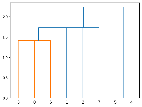
Let’s observe that this population, which only has vertical inheritance, does not have holes. For this purpose, we use the function we created, create_complex, to calculate persistence and the simplex tree.

# Create a Vietoris-Rips complex from the distance matrix, and compute persistent homology.
persistence_esc, simplex_tree_esc = create_complex(hamming_distance_matrix_esc)

Now, let’s visualize the barcode and the persistence diagram.

gd.plot_persistence_barcode(persistence_esc)
gd.plot_persistence_diagram(persistence_esc)

In these plots, we can observe that we only have non-zero Betti numbers for $\beta_0$, indicating that in this population, which only has vertical inheritance, applying persistent homology does not yield 1-holes.

Case Study 2: Introducing Horizontal Gene Transfer

Now, we introduce a horizontal gene transfer event in the simulation. within a subgroup of this population and apply TDA to analyze the resulting genomic data. The introduction of HGT is expected to manifest as 1-dimensional holes ($ H_1 $) in the barcode diagram, distinct from the baseline scenario. These 1-holes indicate the presence of loops or cycles within the data, directly correlating to the HGT events, as they disrupt the simple connectivity pattern observed with vertical inheritance.

To apply persistent homology to a population that includes horizontal gene transfer we first import population_esc_hgt, in which we simulated horizontal transfer among a group of 3 genomes sharing a window of 15 genes.

population_esc_hgt = np.load('https://github.com/carpentries-incubator/topological-data-analysis/raw/gh-pages/files/population_esc_hgt.npy')
population_esc_hgt

array([[0, 1, 0, ..., 0, 1, 0],
       [0, 1, 0, ..., 0, 1, 0],
       [0, 1, 0, ..., 0, 1, 0],
       ...,
       [0, 1, 0, ..., 0, 1, 0],
       [0, 1, 0, ..., 0, 1, 0],
       [0, 1, 0, ..., 0, 1, 0]])

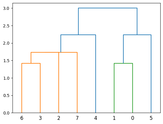
Now the cladogram looks like this:

plot_dendrogram(population_esc_hgt)

Now let’s calculate the Hamming matrix and persistence.

hamming_matrix_esc_hgt = calculate_hamming_matrix(population_esc_hgt)

persistence_esc_hgt, simplex_tree_esc_hgt = create_complex(hamming_matrix_esc_hgt)
persistence_esc_hgt

[(1, (11.0, 14.0)),
 (0, (0.0, inf)),
 (0, (0.0, 9.0)),
 (0, (0.0, 5.0)),
 (0, (0.0, 5.0)),
 (0, (0.0, 3.0)),
 (0, (0.0, 3.0)),
 (0, (0.0, 2.0)),
 (0, (0.0, 2.0))]

We can see that persistence includes a dimension one. Now, let’s visually represent the simplicial complex for a filtration time of 11.

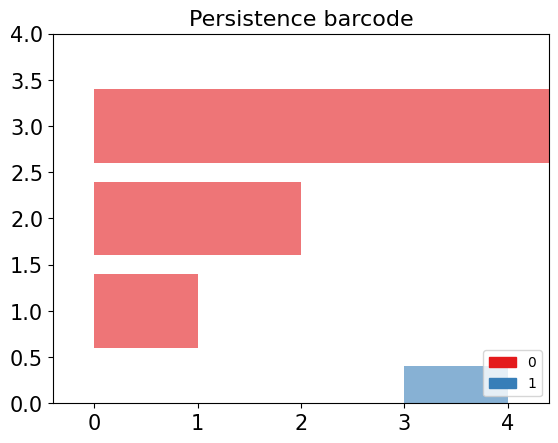
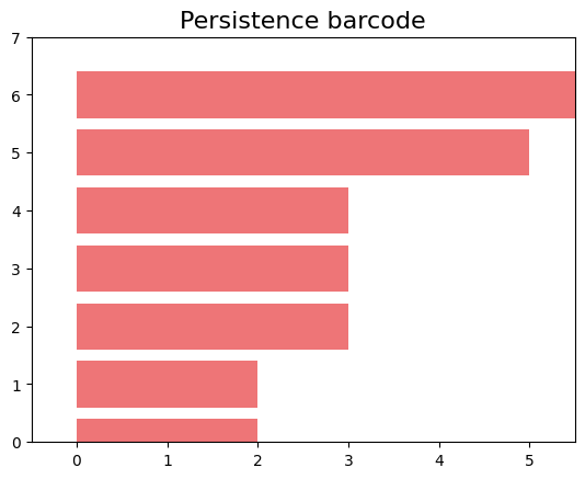
gd.plot_persistence_barcode(persistence_esc_hgt)
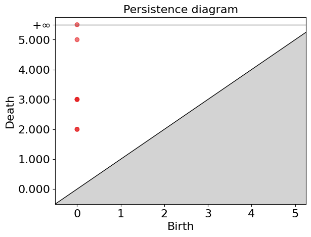
gd.plot_persistence_diagram(persistence_esc_hgt)

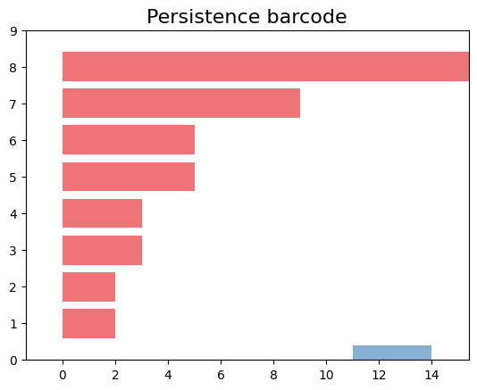
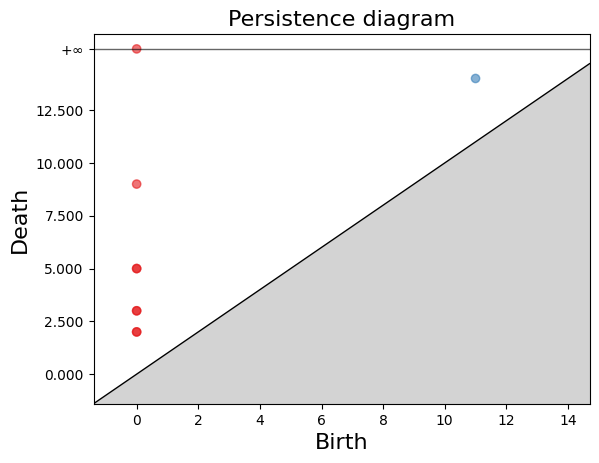
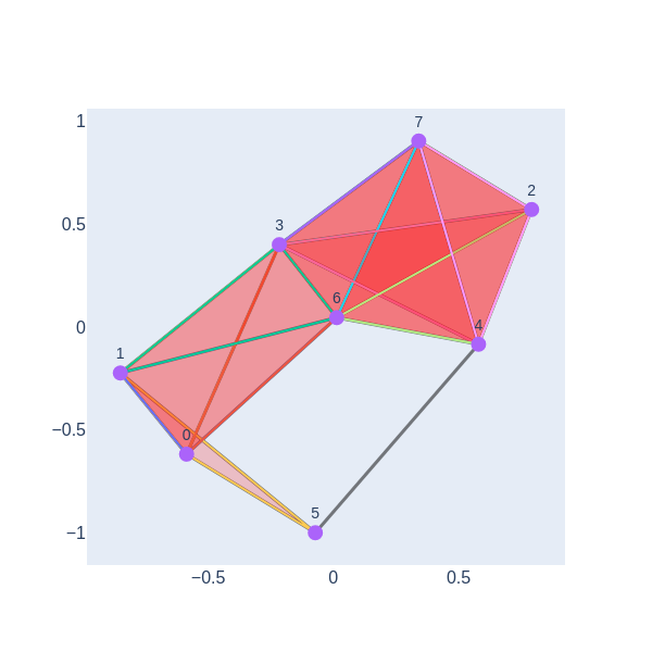
We have a 1-hole born at a distance of 11 and disappears at 14. Let’s geometrically visualize the simplicial complex for a filtration time 11.

visualize_simplicial_complex(simplex_tree_esc_hgt,11)

Persistent Homolgy in the Streptococcus agalactiae genomes

In previous sections, we simulated evolution with
vertical gene transfer and applied persistent homology, showcasing the barcode diagram highlighting connected components. Then, in our second example, we simulated HGT and found some 1-holes. Now, we show an example involving our population of eight S. agalactiae genomes. We want to investigate whether the resistance genes present in the first pangenome of S. agalactiae are the product of vertical inheritance, or other processes could be involved.

Exercise 1(Beginner): Manipulating dataframes

Dataframes Ask ChatPGT or consult stack over flow about the following dataframe functions 1) how to load data in dataframe from a link 2) How to transpose a dataframe

Solution

1) pd.read_csv 2) dataframe.T

First, we will read the S. agalactiae resistance genes that we obtained in the episode Annotating Genomic Data, from the lesson Pangenome Analysis in Prokaryotes.

link="https://raw.githubusercontent.com/carpentries-incubator/topological-data-analysis/gh-pages/files/agalactiae_card_full.tsv"
# Load the dataframe with the new link
df_new = pd.read_csv(link, sep='\t')
# Transpose the dataframe such that column names become row indices and row indices become column names
df_transposed_new = df_new.set_index(df_new.columns[0]).T
df_transposed_new

aro	3000005	3000010	3000013	3000024	3000025	3000026	3000074	3000090	3000118	3000124
agalactiae_18RS21	1	1	1	1	1	1	1	1	1	1
agalactiae_2603V	1	1	1	1	1	1	1	1	1	1
agalactiae_515	1	0	1	1	1	1	1	1	1	1
agalactiae_A909	1	1	1	0	1	1	1	1	1	1
agalactiae_CJB111	1	0	1	0	1	1	1	1	1	1
agalactiae_COH1	1	0	1	1	1	1	1	1	1	1
agalactiae_H36B	1	1	1	1	1	1	1	1	1	1
agalactiae_NEM316	1	0	1	0	1	1	1	1	1	1
8 rows × 1443 columns

Now, we will obtain the values from the data frame.

values=df_transposed_new.iloc[:,:].values

array([[1, 1, 1, ..., 1, 1, 1],
       [1, 1, 1, ..., 1, 1, 1],
       [1, 0, 1, ..., 1, 1, 1],
       ...,
       [1, 0, 1, ..., 1, 1, 1],
       [1, 1, 1, ..., 1, 1, 1],
       [1, 0, 1, ..., 1, 1, 1]])

Now, we extract the names of the Strains from the table.

strains=list(df_transposed_new.index)
strains_names = [s.replace('agalactiae_', '') for s in strains]
strains_names

['18RS21', '2603V', '515', 'A909', 'CJB111', 'COH1', 'H36B', 'NEM316']

Exercise 2(Beginner): Persistent homology of S. agalactiae resistome

Fill in the blanks with the following parameters to calculate the persistent homology of the S. agalactiae resistome.
hamming_matrix_3, values, calculate_hamming_matrix, create_complex
hamming_matrix_3 = __________(_____)
persistence3, simplex_tree3 = ________(_______)
persistence3
Solution
hamming_matrix_3 = calculate_hamming_matrix(values)  
persistence3, simplex_tree3 = create_complex(hamming_matrix_3)
persistance3  
persistance3 will store this data.
[(1, (268.0, 280.0)),
(0, (0.0, inf)),
(0, (0.0, 290.0)),
(0, (0.0, 272.0)),
(0, (0.0, 264.0)),
(0, (0.0, 263.0)),
(0, (0.0, 258.0)),
(0, (0.0, 248.0)),
(0, (0.0, 164.0))]

Exercise 3(Beginner): Plot the persistent barcode of S. agalactiae resistome

Chose the right parameters to plot the persistence diagram of S. agalactiae resistome.

Which one is the correct answer?

A)
gd.plot_persistence_barcode(persistence3)
B)
gd.plot_persistence_diagram(persistence3, legend=True)
C)
gd.plot_persistence_barcode(persistence3, legend=True)
Solution

C)
gd.plot_persistence_barcode(persistence3, legend=True)

Exercise 4(Intermediate): Are the S_agalaciae resistome product of vertical inheritance?

Based on visualization of the simplicial complex at time 270. Which evolutionary processes may be involved in S. agalactiae resistome?
visualize_simplicial_complex(simplex_tree3,270,strains_names)
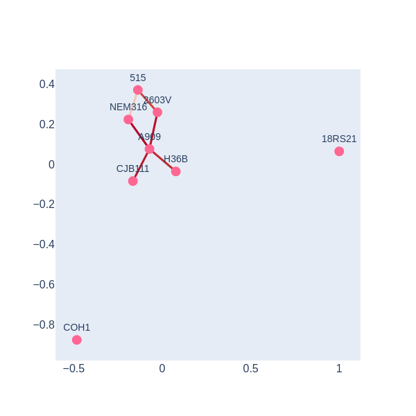
Solution

There is a 1-holes in the barcode diagram, so there is preliminary evidence that this resistome was not acquired only via vertical inheritance

By employing TDA and persistent homology, we gain a powerful lens through which to observe and understand the impact of HGT on bacterial genomes. This approach not only underscores the utility of TDA in genomic research but also highlights its potential to uncover intricate gene transfer patterns that are critical for understanding bacterial evolution and antibiotic resistance.

Key Points

Horizontal Gene Transfer (HGT) is a phenomenon where an organism transfers genetic material to another one that is not its descendant.

1-holes can detect HGT.

Persistence Simplices gives rise to Gene Families

Overview

Teaching: 30 min
Exercises: 20 min

Questions

How can I apply TDA to describe Pangenomes?

How can persistence simplices be related to gene families?

Objectives

Describe Pangenomes using Gudhi

Finding persistence families of genes

Explore the change of gene families by varying the distance parameter

Persistent approach to pangenomics

We will work with the four mini-genomes of episode Measuring Sequence Similarity. First, we need to import all the libraries that we will use.

import pandas as pd
from matplotlib import cm
import numpy as np
import gudhi
import time
import os  

Now, we need to read the mini-genomes.blast file that we produced in the episode of Measuring Sequence Similarity.

url = "https://raw.githubusercontent.com/carpentries-incubator/pangenomics/gh-pages/files/mini-genomes.blast"
blastE = pd.read_csv(url, sep='\t', names=['qseqid', 'sseqid', 'evalue'])
 

Obtain a list of the unique genes.

qseqid_unique=pd.unique(blastE['qseqid'])
sseqid_unique=pd.unique(blastE['sseqid'])
genes = pd.unique(np.append(qseqid_unique, sseqid_unique))

We have 43 unique genes, we can check it as follows.

len(genes)

Also, we will need a list of the unique genomes in our database. First, we convert to a data frame object the list of genes, then we split each gene in the genome and gen part, and finally we obtain a list of the unique genomes and save it in the object genomes.

df_genes=pd.DataFrame(genes, columns=['Genes'])
df_genome_genes=df_genes["Genes"].str.split("|", n = 1, expand = True)
df_genome_genes.columns= ["Genome", "Gen"]
genomes=pd.unique(df_genome_genes['Genome'])
genomes=list(genomes)
genomes

['2603V', '515', 'A909', 'NEM316']

To use the gudhi packages, we need a distance matrix. In this case, we will use the evalue as the measure of how similar the genes are. First, we will process the blastE data frame to a list and then we will convert it into a matrix object.

distance_list = blastE[ blastE['qseqid'].isin(genes) & blastE['sseqid'].isin(genes)]
distance_list.head()

  qseqid	              sseqid	              evalue
2603V|GBPINHCM_01420	NEM316|AOGPFIKH_01528	4.110000e-67
2603V|GBPINHCM_01420	A909|MGIDGNCP_01408	4.110000e-67
2603V|GBPINHCM_01420	515|LHMFJANI_01310	4.110000e-67
2603V|GBPINHCM_01420	2603V|GBPINHCM_01420	4.110000e-67
2603V|GBPINHCM_01420	A909|MGIDGNCP_01082	1.600000e+00

As we saw in episode Measuring Sequence Similarity, the BLAST E-value represents the possibility of finding a match with a similar score in a database. By default, BLAST considers a maximum score for the E-value 10, but in this case, there are hits of low quality. If two sequences are not similar or if the E-value is bigger than 10, then BLAST does not save this score. In order to have something like a distance matrix we will fill the E-value of the sequence for which we do not have a score. To do this, we will use the convention that an E-value equal to 5 is too big and that the sequences are not similar at all.

MaxDistance = 5.0000000

# reshape long to wide
matrixE = pd.pivot_table(distance_list,index = "qseqid",values = "evalue",columns = 'sseqid')
matrixE.iloc[1:5,1:5]

sseqid	2603V|GBPINHCM_00065	2603V|GBPINHCM_00097	2603V|GBPINHCM_00348	2603V|GBPINHCM_00401
qseqid				
2603V|GBPINHCM_00065	1.240000e-174	NaN	NaN	NaN
2603V|GBPINHCM_00097	NaN	9.580000e-100	NaN	NaN
2603V|GBPINHCM_00348	NaN	NaN	0.0	NaN
2603V|GBPINHCM_00401	NaN	NaN	NaN	2.560000e-135

matrixE2=matrixE.fillna(MaxDistance)
matrixE2.iloc[0:4,0:4]

sseqid	2603V|GBPINHCM_00065	2603V|GBPINHCM_00097	2603V|GBPINHCM_00348	2603V|GBPINHCM_00401
qseqid				
2603V|GBPINHCM_00065	1.240000e-174	5.000000e+00	5.0	5.000000e+00
2603V|GBPINHCM_00097	5.000000e+00	9.580000e-100	5.0	5.000000e+00
2603V|GBPINHCM_00348	5.000000e+00	5.000000e+00	0.0	5.000000e+00
2603V|GBPINHCM_00401	5.000000e+00	5.000000e+00	5.0	2.560000e-135

We need to have an object with the names of the columns of the matrix that we will use later.

name_columns = matrixE2.columns
name_columns

Index(['2603V|GBPINHCM_00065', '2603V|GBPINHCM_00097', '2603V|GBPINHCM_00348',
       '2603V|GBPINHCM_00401', '2603V|GBPINHCM_00554', '2603V|GBPINHCM_00748',
       '2603V|GBPINHCM_00815', '2603V|GBPINHCM_01042', '2603V|GBPINHCM_01226',
       '2603V|GBPINHCM_01231', '2603V|GBPINHCM_01420', '515|LHMFJANI_00064',
 ...,
       'NEM316|AOGPFIKH_01341', 'NEM316|AOGPFIKH_01415',
       'NEM316|AOGPFIKH_01528', 'NEM316|AOGPFIKH_01842'],
      dtype='object', name='sseqid')

Finally, we need the distance matrix as a numpy array.

DistanceMatrix = matrixE2.to_numpy()
DistanceMatrix

array([[1.24e-174, 5.00e+000, 5.00e+000, ..., 5.00e+000, 5.00e+000,
        5.00e+000],
       [5.00e+000, 9.58e-100, 5.00e+000, ..., 5.00e+000, 5.00e+000,
        5.00e+000],
       [5.00e+000, 5.00e+000, 0.00e+000, ..., 5.00e+000, 5.00e+000,
        5.00e+000]

Now, we want to construct the Vietoris-Rips complex associated with the genes with respect to the distance matrix that we obtained. In the episode Introduction Topological Data Analysis we saw that to construct the Vietoris-Rips complex we need to define a distance parameter or threshold, so the points within a distance less than or equal to the threshold get connected in the complex. The threshold is defined by the argument max_edge_length, and we will use here the value 2.

max_edge_length = 2
# Rips complex with the distance matrix
start_time = time.time()
ripsComplex = gudhi.RipsComplex(
    distance_matrix = DistanceMatrix, 
    max_edge_length = max_edge_length
)
print("The Rips complex was created in %s" % (time.time() - start_time) )

The Rips complex was created in 0.00029540061950683594

Discussion: Changing the maximum dimension of the edges

To create the Rips Complex, we fixed that the maximum edge length was 2. What happens if we use a different parameter?
For example, if we use max_edge_lenght=1. Do you expect to have more simplices? Why?

Solution

If we use a different max_edge_length we will obtain a differente filtration with less or more simplices. In the case of max_edge_lenght=1 we will have less simplices because we stop the creation of simplices when the radius of the balls around the simplices are 1.

As we see in the previous episodes, we now need a filtration. We will use the gudhi function create_simplex_tree to obtain the filtration associated with the Rips complex. We need to specify the argument max_dimension, this argument is the maximum dimension of the simplicial complex that we will obtain. If it is for example 4, this means that we will obtain gene families with at most 4 genes. In this example, we will use 8 as the maximum dimension so we can have families with at most 2 genes from each genome or 8 different genes.

Note

For complete genomes, the maximum dimension of the simplicial complex needs to be carefully chosen because the computation in Python is demanding in terms of system resources. For example, with 4 complete genomes the maximum dimension that we can compute is 5.

start_time = time.time()
simplexTree = ripsComplex.create_simplex_tree(
    max_dimension = 8)
print("The filtration of the Rips complex was created in %s" % (time.time() - start_time))

The filtration of the Rips complex was created in 0.001073598861694336

With the persistence() function, we will obtain the persistence of each simplicial complex.

start_time = time.time()
persistence = simplexTree.persistence()  
print("The persistente diagram of the Rips complex was created in %s" % (time.time() - start_time))

The persistente diagram of the Rips complex was created in 0.006387233734130859

We can print the birth time of the simplices. If we check the output of the following, we can see the simplices with how many vertices they have and with the birth time of each.

result_str = 'Rips complex of dimension ' + repr(simplexTree.dimension())
print(result_str)
fmt = '%s -> %.2f'
for filtered_value in simplexTree.get_filtration():
    print(tuple(filtered_value))

Rips complex of dimension 7
([0], 0.0)
([1], 0.0)
([2], 0.0)
([3], 0.0)
([4], 0.0)
([5], 0.0)
([6], 0.0)
([7], 0.0)
...

simplexTree.dimension(), simplexTree.num_vertices(), simplexTree.num_simplices()

(7, 43, 467)

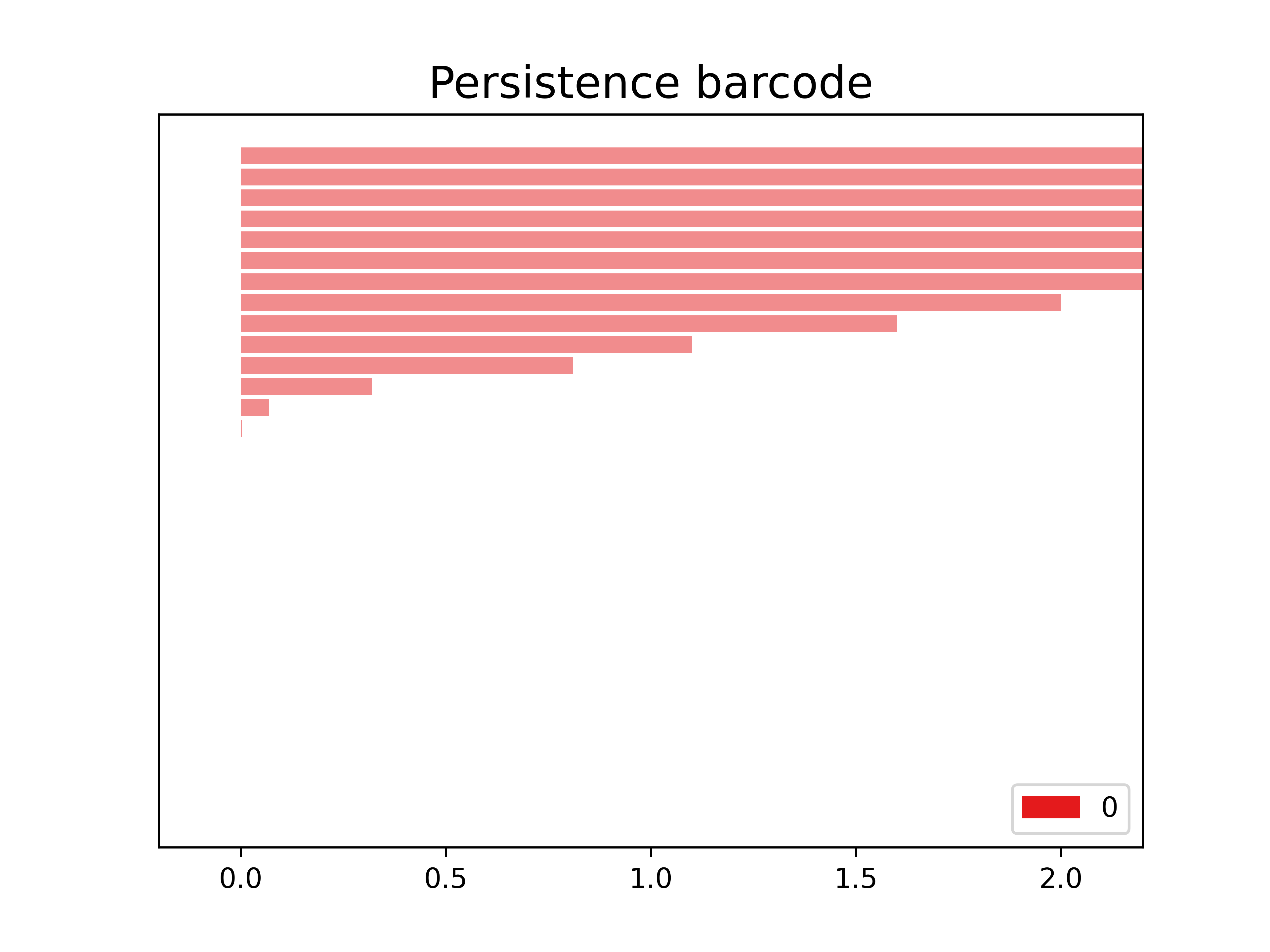
The following is the barcode of the filtration that we created. We observe in this case that we only have objects in dimension 0.

start_time = time.time()
gudhi.plot_persistence_barcode(
    persistence = persistence, 
    alpha = 0.5,
    colormap = cm.Set2.colors
)
print("Bar code diagram was created in %s" % (time.time() - start_time))

Bar code diagram was created in 0.05829215049743652

The following function allows us to obtain the dimension of the simplices.

def dimension(list):
    return (len(list[0])-1, list[1])

We filter according to the dimension function: it orders the simplices from largest dimension to smallest and then from longest birth time to smallest.

all_simplex_sorted_dim_1 = sorted(simplexTree.get_filtration(), key = dimension, reverse = True)
all_simplex_sorted_dim_1 

[([4, 9, 15, 18, 25, 30, 37, 39], 0.014),
 ([4, 9, 15, 18, 25, 30, 37], 0.014),
 ([4, 9, 15, 18, 25, 30, 39], 0.014),
 ([4, 9, 15, 18, 25, 37, 39], 0.014),
...
 ([35], 0.0),
 ([36], 0.0),
 ([37], 0.0),
 ([38], 0.0),
 ([39], 0.0),
 ([40], 0.0),
 ([41], 0.0),
 ([42], 0.0)]

Obtain the persistence of each simplex.

d_simplex_time = dict()
d_simplex_const = dict()
names = []
for tuple_simple in all_simplex_sorted_dim_1:
    list_aux = []
    if len(tuple_simple[0])-1 == simplexTree.dimension(): 
        t_birth = tuple_simple[1]
        t_death = max_edge_length
        d_simplex_time[tuple(tuple_simple[0])] = (t_birth,t_death)
        list_aux = tuple([name_columns[tuple_simple[0][i]] for i in range(len(tuple_simple[0]))])
        d_simplex_const[list_aux] = (t_birth,t_death)
    else:
        t_birth = tuple_simple[1] 
        t_death = max_edge_length
        for simplex in d_simplex_time.keys():
            if set(tuple_simple[0]).issubset(set(simplex)):
                t_death = d_simplex_time[simplex][0] 
        d_simplex_time[tuple(tuple_simple[0])] = (t_birth,t_death)
        list_aux = tuple([name_columns[tuple_simple[0][i]] for i in range(len(tuple_simple[0]))])
        d_simplex_const[list_aux] = (t_birth,t_death) 

We can save the name of the simplices, i.e. the keys in the object d_simplex_const, in a list called simplices.

simplices = list()
simplices = list(d_simplex_const.keys())

Now, we want an object with the information on how many genes of each genome are in each family.

bool_gen = dict()
genes_contains = dict()
num_new_columns = len(genomes)
for simplex in simplices:
    genes_contains = dict()
    genes_contains = {'2603V': 0, '515': 0, 'A909': 0, 'NEM316': 0}
    for i in range(len(simplex)):
        for genoma in genomes:
            if genoma in simplex[i]:
                genes_contains[genoma] = genes_contains[genoma] +1
    for gen in genomes:
        if gen not in genes_contains.keys():
            genes_contains[gen] = 0
    bool_gen[simplex] = genes_contains
bool_gen

The bool_gen numbers looks like:

{('2603V|GBPINHCM_00554',
  '2603V|GBPINHCM_01231',
  '515|LHMFJANI_00548',
  '515|LHMFJANI_01178',
  'A909|MGIDGNCP_00580',
  'A909|MGIDGNCP_01268',
  'NEM316|AOGPFIKH_00621',
  'NEM316|AOGPFIKH_01341'): {'2603V': 2, '515': 2, 'A909': 2, 'NEM316': 2},
 ('2603V|GBPINHCM_00554',
  '2603V|GBPINHCM_01231',
  '515|LHMFJANI_00548',
  '515|LHMFJANI_01178',
  'A909|MGIDGNCP_00580',
  'A909|MGIDGNCP_01268',
  'NEM316|AOGPFIKH_00621'): {'2603V': 2, '515': 2, 'A909': 2, 'NEM316': 1},
...
('NEM316|AOGPFIKH_00855',): {'2603V': 0, '515': 0, 'A909': 0, 'NEM316': 1},
 ('NEM316|AOGPFIKH_01341',): {'2603V': 0, '515': 0, 'A909': 0, 'NEM316': 1},
 ('NEM316|AOGPFIKH_01415',): {'2603V': 0, '515': 0, 'A909': 0, 'NEM316': 1},
 ('NEM316|AOGPFIKH_01528',): {'2603V': 0, '515': 0, 'A909': 0, 'NEM316': 1},
 ('NEM316|AOGPFIKH_01842',): {'2603V': 0, '515': 0, 'A909': 0, 'NEM316': 1}}

How can we read the object bool_gen?

We have a dictionary of dictionaries. Every key in the dictionary is a family and in the values, we have how many genes are from each genome in each family.

Now, we want to obtain a dataframe with information on the time of births, death, and persistence of every simplex (i.e. every family). First, we will obtain this information from our object d_simplex_time and we will save it in tree lists.

births = []
deaths = []
persistent_times = []
for values in d_simplex_time.values():
    births.append(values[0])
    deaths.append(values[1])
    persistent_times.append(values[1]-values[0])

Now that we have the information we will save it in the dataframe simplex_list

data = {
    't_birth': births,
    't_death': deaths,
    'persistence': persistent_times
}
simplex_list = pd.DataFrame(index = simplices, data = data)
simplex_list.head(4)

	t_birth	t_death	persistence
(2603V|GBPINHCM_00554, 2603V|GBPINHCM_01231, 515|LHMFJANI_00548, 515|LHMFJANI_01178, A909|MGIDGNCP_00580, A909|MGIDGNCP_01268, NEM316|AOGPFIKH_00621, NEM316|AOGPFIKH_01341)	0.014	2.000	1.986
(2603V|GBPINHCM_00554, 2603V|GBPINHCM_01231, 515|LHMFJANI_00548, 515|LHMFJANI_01178, A909|MGIDGNCP_00580, A909|MGIDGNCP_01268, NEM316|AOGPFIKH_00621)	0.014	0.014	0.000
(2603V|GBPINHCM_00554, 2603V|GBPINHCM_01231, 515|LHMFJANI_00548, 515|LHMFJANI_01178, A909|MGIDGNCP_00580, A909|MGIDGNCP_01268, NEM316|AOGPFIKH_01341)	0.014	0.014	0.000
(2603V|GBPINHCM_00554, 2603V|GBPINHCM_01231, 515|LHMFJANI_00548, 515|LHMFJANI_01178, A909|MGIDGNCP_00580, NEM316|AOGPFIKH_00621, NEM316|AOGPFIKH_01341)	0.014	0.014	0.000

Finally, we want the data frame with complete information, so we will concatenate the objects simplex_list and bool_gen in a convenient way.

aux_simplex_list = simplex_list
for gen in genomes:
    data = dict()
    dataFrame_aux = []
    for simplex in simplices:
        data[simplex] = bool_gen[simplex][gen]
    dataFrame_aux = pd.DataFrame.from_dict(data, orient='index', columns = [str(gen)])
    aux_simplex_list=pd.concat([aux_simplex_list, dataFrame_aux], axis = 1)
aux_simplex_list.head(4)

	t_birth	t_death	persistence	2603V	515	A909	NEM316
(2603V|GBPINHCM_00554, 2603V|GBPINHCM_01231, 515|LHMFJANI_00548, 515|LHMFJANI_01178, A909|MGIDGNCP_00580, A909|MGIDGNCP_01268, NEM316|AOGPFIKH_00621, NEM316|AOGPFIKH_01341)	0.014	2.000	1.986	2	2	2	2
(2603V|GBPINHCM_00554, 2603V|GBPINHCM_01231, 515|LHMFJANI_00548, 515|LHMFJANI_01178, A909|MGIDGNCP_00580, A909|MGIDGNCP_01268, NEM316|AOGPFIKH_00621)	0.014	0.014	0.000	2	2	2	1
(2603V|GBPINHCM_00554, 2603V|GBPINHCM_01231, 515|LHMFJANI_00548, 515|LHMFJANI_01178, A909|MGIDGNCP_00580, A909|MGIDGNCP_01268, NEM316|AOGPFIKH_01341)	0.014	0.014	0.000	2	2	2	1
(2603V|GBPINHCM_00554, 2603V|GBPINHCM_01231, 515|LHMFJANI_00548, 515|LHMFJANI_01178, A909|MGIDGNCP_00580, NEM316|AOGPFIKH_00621, NEM316|AOGPFIKH_01341)	0.014	0.014	0.000	2	2	1	2

In this data frame, we can see the history of the formation of families (simplices) at the different birth and death times. If we filter at t_death=2we can see only the families that we remain with in the end.

Exercise 1(Beginner): Partitioning the pangenome

Filter the table by t_death=2, at this point in the filtration, which families are in each partition Core, Shell and Cloud? How many of these are single-copy core families?

Solution

We can filter as follows:

aux_simplex_list[aux_simplex_list['t_death']==2]

	t_birth	t_death	persistence	2603V	515	A909	NEM316
(2603V|GBPINHCM_00554, 2603V|GBPINHCM_01231, 515|LHMFJANI_00548, 515|LHMFJANI_01178, A909|MGIDGNCP_00580, A909|MGIDGNCP_01268, NEM316|AOGPFIKH_00621, NEM316|AOGPFIKH_01341)	1.400000e-02	2.0	1.986	2	2	2	2
(2603V|GBPINHCM_00401, 515|LHMFJANI_00394, 515|LHMFJANI_01625, A909|MGIDGNCP_00405, NEM316|AOGPFIKH_00403, NEM316|AOGPFIKH_01842)	1.300000e+00	2.0	0.700	1	2	1	2
(2603V|GBPINHCM_01042, 2603V|GBPINHCM_01420, 515|LHMFJANI_01310, A909|MGIDGNCP_01408, NEM316|AOGPFIKH_01528)	1.600000e+00	2.0	0.400	2	1	1	1
(2603V|GBPINHCM_00065, 515|LHMFJANI_00064, A909|MGIDGNCP_00064, A909|MGIDGNCP_00627, NEM316|AOGPFIKH_00065)	8.600000e-02	2.0	1.914	1	1	2	1
(2603V|GBPINHCM_00348, 515|LHMFJANI_00342, A909|MGIDGNCP_00352, NEM316|AOGPFIKH_00350, NEM316|AOGPFIKH_01341)	3.000000e-03	2.0	1.997	1	1	1	2
(2603V|GBPINHCM_01042, A909|MGIDGNCP_01082, A909|MGIDGNCP_01408, NEM316|AOGPFIKH_01528)	1.600000e+00	2.0	0.400	1	0	2	1
(2603V|GBPINHCM_00748, 515|LHMFJANI_00064, A909|MGIDGNCP_00064, NEM316|AOGPFIKH_00065)	8.300000e-01	2.0	1.170	1	1	1	1
(2603V|GBPINHCM_00097, 515|LHMFJANI_00097, A909|MGIDGNCP_00096, NEM316|AOGPFIKH_00098)	9.580000e-100	2.0	2.000	1	1	1	1
(2603V|GBPINHCM_00815, 515|LHMFJANI_00781, A909|MGIDGNCP_00877, NEM316|AOGPFIKH_00855)	0.000000e+00	2.0	2.000	1	1	1	1
(2603V|GBPINHCM_00748, 2603V|GBPINHCM_01042, A909|MGIDGNCP_01082)	2.000000e+00	2.0	0.000	2	0	1	0
(2603V|GBPINHCM_00748, 2603V|GBPINHCM_01042)	2.000000e+00	2.0	0.000	2	0	0	0
(2603V|GBPINHCM_00748, A909|MGIDGNCP_01082)	2.000000e+00	2.0	0.000	1	0	1	0
(515|LHMFJANI_01625, A909|MGIDGNCP_01221)	1.100000e+00	2.0	0.900	0	1	1	0
(515|LHMFJANI_01130, A909|MGIDGNCP_01221)	1.310000e-85	2.0	2.000	0	1	1	0
(A909|MGIDGNCP_01343, NEM316|AOGPFIKH_01415)	7.890000e-143	2.0	2.000	0	0	1	1
(2603V|GBPINHCM_01226,)	0.000000e+00	2.0	2.000	1	0	0	0

Partition	Num. of Families
Core	8
Shell	6
Cloud	2

Single-copy core families: 3

Excercise 2(Beginner): Looking for functional families

In the episode Measuring Sequence Similarity we saw that the genes 2603V|GBPINHCM_01420, 515|LHMFJANI_01310, A909|MGIDGNCP_01408, and NEM316|AOGPFIKH_01528 make the functional family 30S ribosomal protein. Look for these genes in the aux_simplex_list. Are they in the same family? Are there other genes in this family?

Solution

Yes, they are in the same family, but there is one more gene in this family, the gene 2603V|GBPINHCM_01042.

Exercise 3(Intermediate): Changing the dimension of the simplices

When we create the object simplexTree we define that the maximum dimension of the simplices was 8. Change this parameter to 3.
With the new parameter, how many simplices do you obtain? And edges? If you run all the code with this new parameter and filter again by t_death = 2, what happens with the partitions? How many families do you have?
Solution
start_time = time.time()
simplexTree = ripsComplex.create_simplex_tree(
   max_dimension = 3)
persistence = simplexTree.persistence()
simplexTree.dimension(), simplexTree.num_vertices(), simplexTree.num_simplices()
(3, 43, 364)
Now we have less simplices, we have 364 simplices.

When we filter by t_death = 2, we obtain 111 families because some families share genes.

Key Points

Pangenomes can be described using TDA

Persistence simplices are related to the gene families of a Pangenome

Persistence simplices can be used to find some funtional families

Other Resources

Overview

Teaching: 10 min
Exercises: 10 min

Questions

What other tools are available in TDA?

What are the limitations of those tools?

Objectives

Explore other tools in R and Python for TDA and understand their limitations.

Python: Giotto-TDA

Giotto-TDA is a Python toolbox for TDA. This tool does not accept point clouds or generate barcodes. However, it can store all the information from a barcode in a variable for later plotting using another tool.

R: tdaverse

The tdaverse repository contains a list of R tools for performing TDA. The packages simplextree, ripserr, and ggtda can carry out almost the same functions as the GUDHI package presented in the episodes.

Wrap up

Carpentries Philosophy

A good lesson should be as complete and clear that becomes easy to teach by any instructor. Carpentries lessons are developed for the community, and now you are part of us. This lesson is being developed and we are sure that you can collaborate and help us improve it.

Key Points

Giotto-TDA and tdaverse are other resources to learn TDA

Topological Data Analysis for Pangenomics

Introduction to Topological Data Analysis

Overview

Topological data analysis

Simplex

Simplex

Mathematical definition

Simplicial complex

Simplicial complex

Mathematical definition

Exercise 1(Beginner): Identify the simplices

Solution

Čech and (Vietoris)-Rips complexes

Vietoris complex

Mathematical definition

Čech complex

Mathematical definition

Note

Simplicial homology

Exercise 2(Beginner): Identify Betti numbers

Solution

Filtration

Filtration

Mathematical definition

Exercise 3(Intermediate): Calculate the Betti numbers.

Solution

Persistence Diagram

Barcode Diagram

App to play

Exercise 4(Advanced): Using the app example

Solution

Key Points

Computational Tools for TDA

Overview

Introduction to GUDHI and Simplicial Homology

Example 1: SimplexTree and Manual Filtration

Create SimplexTree

Insert simplex

Note

Persistence

Plot the persistence diagram

Plot the barcode

Exercise 1(Intermediate): Creating a Manually Filtered Simplicial Complex.

Solution

Example 2: Rips complex from datasets

Generate dataset

Plot dataset

Create Rips complex

Simplicial homology

Plots the persistence diagram and barcode

Example 3: Rips complex from datasets

Exercise 2(Intermediate): Constructing a Torus and Analyzing Persistent Homology.

Solution

FIXME

Key Points

Detecting horizontal gene transfer

Overview

Introduction to Horizontal Gene Transfer

Know more: Mechanisms of HGT

Extra content

Understanding Persistent Homology in the Context of HGT:

Know more: TDA in genomics

Importing Libraries

Defining Fuctions

Case Study 1: Vertical Inheritance in a Simulated Population

Case Study 2: Introducing Horizontal Gene Transfer

Persistent Homolgy in the Streptococcus agalactiae genomes

Exercise 1(Beginner): Manipulating dataframes

Solution

Exercise 2(Beginner): Persistent homology of S. agalactiae resistome

Solution

Exercise 3(Beginner): Plot the persistent barcode of S. agalactiae resistome

Solution

Exercise 4(Intermediate): Are the S_agalaciae resistome product of vertical inheritance?

Solution

Key Points

Persistence Simplices gives rise to Gene Families

Overview

Persistent approach to pangenomics

Discussion: Changing the maximum dimension of the edges