Detecting horizontal gene transfer

Overview

Teaching: 30 min
Exercises: 30 min

Questions

How can I detect HGT with TDA?

Objectives

Understand hierarchical data does not have 1-holes

Compute the Hamming matrix for applying Persistent Homology.

Introduction to Horizontal Gene Transfer

Horizontal gene transfer (HGT) is a process through which organisms transfer genetic material to each other in a non-traditional way without sexual reproduction. This phenomenon is particularly common among bacteria. Unlike vertical gene transfer, where genetic material is inherited from parents to offspring, HGT allows bacteria to acquire new genes directly from other organisms, potentially even from different species.

HGT is crucial in the rapid spread of antibiotic-resistant genes among bacteria, enabling them to quickly adapt to new environments and survive in the presence of antibiotics. Antibiotic resistance genes can be located on plasmids, small DNA molecules that can be easily transferred between bacteria, accelerating the spread of resistance. The horizontal transfer of antibiotic-resistance genes poses a significant challenge to global public health. It leads to the development and spread of “superbugs” resistant to multiple antibiotics, complicating the treatment of common infections and increasing mortality.

Know more: Mechanisms of HGT

Extra content

You can read more about Horizontal Gene Transfer in this Wikipedia Article. For instance, the main mechanisms of HGT are the following:

Transformation: Direct DNA uptake from the environment.

Transduction: Transfer of genes by bacteriophages (viruses that infect bacteria).

Conjugation: Transfer of genetic material between bacteria through direct contact, usually via a structure known as a pilus.

Understanding Persistent Homology in the Context of HGT:

Topological data analysis (TDA), particularly persistent homology, allows for identifying complex patterns and structures in large genomic datasets, facilitating the detection of HGT of antibiotic resistance genes. Hierarchical data does not have holes in higger dimensions when represented with a Vietoris Rips complex. A population not experiencing horizontal gene transfer and where no mutations are allowed in the same site show non-empty homology only at $ \H_0 $. Remember, $ \H_0 $ in the barcode diagram indicates the presence of connected components.

Here, we will study study cases, 1) we will show persistent homology in vertical inheritance, 2) we will study a simulation of Horizontal Gene Transfer, and 3)In the exercises, we will calculate the persistent homology of the resistant genes from Streptococcus agalactiae that we obtained in the episode Annotating Genomic Data, from the lesson Pangenome Analysis in Prokaryotes. In all three cases, we are going to need first to import some libraries, then to define functions, and finally to call them to visualize the data.

Know more: TDA in genomics

To learn more about applications of TDA in genomics, consult the Rabadan book Topological Data Analysis for Genomics

Importing Libraries

To begin, we will import the necessary packages.

import numpy as np
import pandas as pd
import seaborn as sns
import matplotlib.pyplot as plt
from scipy.cluster.hierarchy import dendrogram, linkage
import gudhi as gd
from scipy.spatial.distance import hamming

import plotly.graph_objs as go
import networkx as nx
import plotly.graph_objects as go
import plotly.io as pio

Defining Fuctions

The function calculate_hamming_matrix calculates a Hamming distance matrix from an array where the columns are genes and the rows are genomes. The hamming distance counts how many differences are in two strings. We have created several hamming distance functions in the episode functions.

# Let's assume that "population" is a numpy ndarray with your genomes as rows.
def calculate_hamming_matrix(population):
    # Number of genomes
    num_genomes = population.shape[0]
    # Create an empty matrix for Hamming distances
    hamming_matrix = np.zeros((num_genomes, num_genomes), dtype=int)
   # Calculate the Hamming distance between each pair of genomes
    for i in range(num_genomes):
        for j in range(i+1, num_genomes):  # j=i+1 to avoid calculating the same distance twice
            # The Hamming distance is multiplied by the number of genes to convert it into an absolute distance
            distance = hamming(population[i], population[j]) * len(population[i])
            hamming_matrix[i, j] = distance
            hamming_matrix[j, i] = distance  # The matrix is symmetric
    
    return hamming_matrix

The create_complex function generates a 3-dimensional Rips simplicial complex and computes persistent homology from a distance matrix.

def create_complex(distance_matrix):
    # Create the Rips simplicial complex from the distance matrix
    rips_complex = gd.RipsComplex(distance_matrix=distance_matrix)
    # Create the simplex tree from the Rips complex with a maximum dimension of 3
    simplex_tree = rips_complex.create_simplex_tree(max_dimension=3)
    # Compute the persistence of the simplicial complex
    persistence = simplex_tree.persistence()
    # Return the persistence diagram or barcode
    return persistence, simplex_tree

Function plot_dendrogram helps visualizing a cladogram.

#### Function for visualization
def plot_dendrogram(data):
    """Plot a dendrogram from the data."""
    linked = linkage(data, 'single')
    dendrogram(linked, orientation='top', distance_sort='descending')
    plt.show()

The visualize_simplicial_complex function creates a graphical representation of a simplicial complex for a given filtration level based on a simplex tree. This function is based on what you learned in the plotting episode in the lesson Introduction to Python.

def visualize_simplicial_complex(simplex_tree, filtration_value, vertex_names=None, save_filename=None, plot_size=1, dpi=600, pos=None):
    G = nx.Graph()
    triangles = []  # List to store triangles (3-nodes simplices)
    
    for simplex, filt in simplex_tree.get_filtration():
        if filt <= filtration_value:
            if len(simplex) == 2:
                G.add_edge(simplex[0], simplex[1])
            elif len(simplex) == 1:
                G.add_node(simplex[0])
            elif len(simplex) == 3:
                triangles.append(simplex)
    
    # Calculate node positions if not provided
    if pos is None:
        pos = nx.spring_layout(G)
    
    # Node trace
    x_values, y_values = zip(*[pos[node] for node in G.nodes()])
    node_labels = [vertex_names[node] if vertex_names else str(node) for node in G.nodes()]
    node_trace = go.Scatter(x=x_values, y=y_values, mode='markers+text', hoverinfo='text', marker=dict(size=14), text=node_labels, textposition='top center', textfont=dict(size=14))
    
    # Edge traces
    edge_traces = []
    for edge in G.edges():
        x0, y0 = pos[edge[0]]
        x1, y1 = pos[edge[1]]
        edge_trace = go.Scatter(x=[x0, x1, None], y=[y0, y1, None], mode='lines', line=dict(width=3, color='rgba(0,0,0,0.5)'))
        edge_traces.append(edge_trace)
    
    # Triangle traces
    triangle_traces = []
    for triangle in triangles:
        x0, y0 = pos[triangle[0]]
        x1, y1 = pos[triangle[1]]
        x2, y2 = pos[triangle[2]]
        triangle_trace = go.Scatter(x=[x0, x1, x2, x0, None], y=[y0, y1, y2, y0, None], fill='toself', mode='lines+markers', line=dict(width=2), fillcolor='rgba(255,0,0,0.2)')
        triangle_traces.append(triangle_trace)
    
    # Configure the layout of the plot
    layout = go.Layout(showlegend=False, hovermode='closest', xaxis=dict(showgrid=False, zeroline=False, tickfont=dict(size=16, family='Arial, sans-serif')), yaxis=dict(showgrid=False, zeroline=False, tickfont=dict(size=16, family='Arial, sans-serif')))
    
    fig = go.Figure(data=edge_traces + triangle_traces + [node_trace], layout=layout)
    
    # Set the figure size
    fig.update_layout(width=plot_size * dpi, height=plot_size * dpi)
    
    # Save the figure if a filename is provided
    if save_filename:
        pio.write_image(fig, save_filename, width=plot_size * dpi, height=plot_size * dpi, scale=1)
    
    # Show the figure
    fig.show()

    return G

Case Study 1: Vertical Inheritance in a Simulated Population

We simulate a bacterial population’s evolution whos inheritance is exclusively by vertical gene transfer (inheritance from parent to offspring). Applying persistent homology to this simulation, we expect a barcode diagram predominantly showing connected components ($ H_0 $), with little to no evidence of higher-dimensional features. This serves as a baseline for understanding the impact of vertical inheritance on genomic data topology.

We proceed to load a numpy array, named population_esc, which contains a resistome of a population with 8 genomes, simulated from a genome with three generations, and in each generation, one genome has 2 offspring. The total number of genes is 505, the initial percentage of 1s is 25%, and the gene gain rate in each generation is 1/505.

population_esc = np.load('https://github.com/carpentries-incubator/topological-data-analysis/raw/gh-pages/files/population_esc.npy')
population_esc

array([[0, 1, 0, ..., 0, 1, 0],
       [0, 1, 0, ..., 0, 1, 0],
       [0, 1, 0, ..., 0, 1, 0],
       ...,
       [0, 1, 0, ..., 0, 1, 0],
       [0, 1, 0, ..., 0, 1, 0],
       [0, 1, 0, ..., 0, 1, 0]])

We calculate its distance matrix using the calculate_hamming_matrix function with the following command:

hamming_distance_matrix_esc= calculate_hamming_matrix(population_esc) #calculate hamming matrix
plot_dendrogram(population_esc) ##plot dendrogram

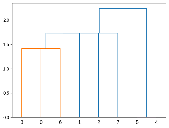
Let’s observe that this population, which only has vertical inheritance, does not have holes. For this purpose, we use the function we created, create_complex, to calculate persistence and the simplex tree.

# Create a Vietoris-Rips complex from the distance matrix, and compute persistent homology.
persistence_esc, simplex_tree_esc = create_complex(hamming_distance_matrix_esc)

Now, let’s visualize the barcode and the persistence diagram.

gd.plot_persistence_barcode(persistence_esc)
gd.plot_persistence_diagram(persistence_esc)

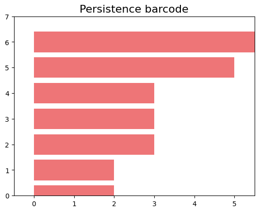
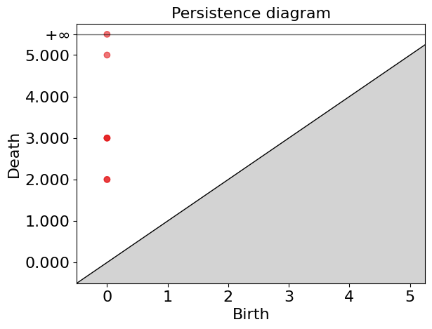
In these plots, we can observe that we only have non-zero Betti numbers for $\beta_0$, indicating that in this population, which only has vertical inheritance, applying persistent homology does not yield 1-holes.

Case Study 2: Introducing Horizontal Gene Transfer

Now, we introduce a horizontal gene transfer event in the simulation. within a subgroup of this population and apply TDA to analyze the resulting genomic data. The introduction of HGT is expected to manifest as 1-dimensional holes ($ H_1 $) in the barcode diagram, distinct from the baseline scenario. These 1-holes indicate the presence of loops or cycles within the data, directly correlating to the HGT events, as they disrupt the simple connectivity pattern observed with vertical inheritance.

To apply persistent homology to a population that includes horizontal gene transfer we first import population_esc_hgt, in which we simulated horizontal transfer among a group of 3 genomes sharing a window of 15 genes.

population_esc_hgt = np.load('https://github.com/carpentries-incubator/topological-data-analysis/raw/gh-pages/files/population_esc_hgt.npy')
population_esc_hgt

array([[0, 1, 0, ..., 0, 1, 0],
       [0, 1, 0, ..., 0, 1, 0],
       [0, 1, 0, ..., 0, 1, 0],
       ...,
       [0, 1, 0, ..., 0, 1, 0],
       [0, 1, 0, ..., 0, 1, 0],
       [0, 1, 0, ..., 0, 1, 0]])

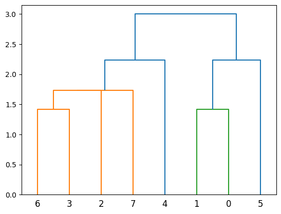
Now the cladogram looks like this:

plot_dendrogram(population_esc_hgt)

Now let’s calculate the Hamming matrix and persistence.

hamming_matrix_esc_hgt = calculate_hamming_matrix(population_esc_hgt)

persistence_esc_hgt, simplex_tree_esc_hgt = create_complex(hamming_matrix_esc_hgt)
persistence_esc_hgt

[(1, (11.0, 14.0)),
 (0, (0.0, inf)),
 (0, (0.0, 9.0)),
 (0, (0.0, 5.0)),
 (0, (0.0, 5.0)),
 (0, (0.0, 3.0)),
 (0, (0.0, 3.0)),
 (0, (0.0, 2.0)),
 (0, (0.0, 2.0))]

We can see that persistence includes a dimension one. Now, let’s visually represent the simplicial complex for a filtration time of 11.

gd.plot_persistence_barcode(persistence_esc_hgt)
gd.plot_persistence_diagram(persistence_esc_hgt)

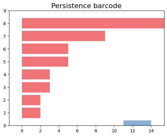
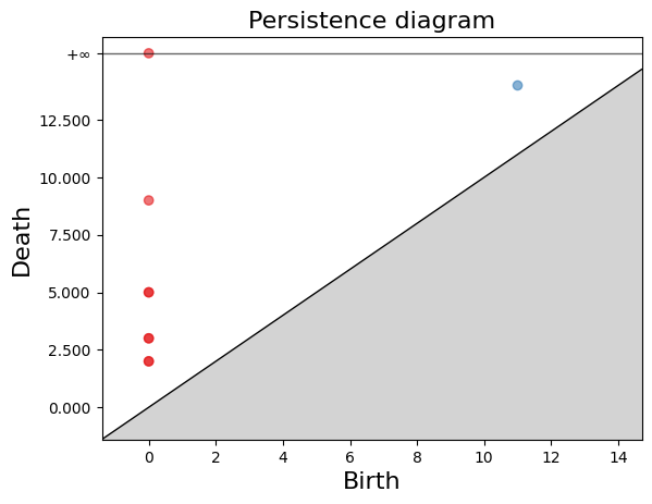
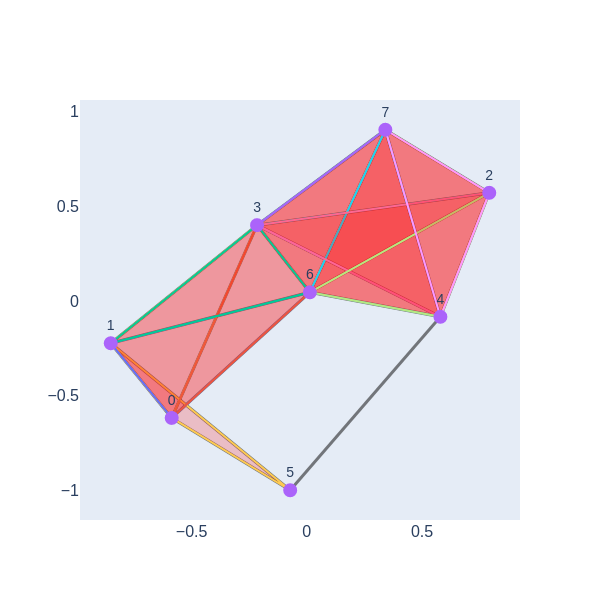
We have a 1-hole born at a distance of 11 and disappears at 14. Let’s geometrically visualize the simplicial complex for a filtration time 11.

visualize_simplicial_complex(simplex_tree_esc_hgt,11)

Persistent Homolgy in the Streptococcus agalactiae genomes

In previous sections, we simulated evolution with
vertical gene transfer and applied persistent homology, showcasing the barcode diagram highlighting connected components. Then, in our second example, we simulated HGT and found some 1-holes. Now, we show an example involving our population of eight S. agalactiae genomes. We want to investigate whether the resistance genes present in the first pangenome of S. agalactiae are the product of vertical inheritance, or other processes could be involved.

Exercise 1(Beginner): Manipulating dataframes

Dataframes Ask ChatPGT or consult stack over flow about the following dataframe functions 1) how to load data in dataframe from a link 2) How to transpose a dataframe

Solution

1) pd.read_csv 2) dataframe.T

First, we will read the S. agalactiae resistance genes that we obtained in the episode Annotating Genomic Data, from the lesson Pangenome Analysis in Prokaryotes.

link="https://raw.githubusercontent.com/carpentries-incubator/topological-data-analysis/gh-pages/files/agalactiae_card_full.tsv"
# Load the dataframe with the new link
df_new = pd.read_csv(link, sep='\t')
# Transpose the dataframe such that column names become row indices and row indices become column names
df_transposed_new = df_new.set_index(df_new.columns[0]).T
df_transposed_new

aro	3000005	3000010	3000013	3000024	3000025	3000026	3000074	3000090	3000118	3000124
agalactiae_18RS21	1	1	1	1	1	1	1	1	1	1
agalactiae_2603V	1	1	1	1	1	1	1	1	1	1
agalactiae_515	1	0	1	1	1	1	1	1	1	1
agalactiae_A909	1	1	1	0	1	1	1	1	1	1
agalactiae_CJB111	1	0	1	0	1	1	1	1	1	1
agalactiae_COH1	1	0	1	1	1	1	1	1	1	1
agalactiae_H36B	1	1	1	1	1	1	1	1	1	1
agalactiae_NEM316	1	0	1	0	1	1	1	1	1	1
8 rows × 1443 columns

Now, we will obtain the values from the data frame.

values=df_transposed_new.iloc[:,:].values

array([[1, 1, 1, ..., 1, 1, 1],
       [1, 1, 1, ..., 1, 1, 1],
       [1, 0, 1, ..., 1, 1, 1],
       ...,
       [1, 0, 1, ..., 1, 1, 1],
       [1, 1, 1, ..., 1, 1, 1],
       [1, 0, 1, ..., 1, 1, 1]])

Now, we extract the names of the Strains from the table.

strains=list(df_transposed_new.index)
strains_names = [s.replace('agalactiae_', '') for s in strains]
strains_names

['18RS21', '2603V', '515', 'A909', 'CJB111', 'COH1', 'H36B', 'NEM316']

Exercise 2(Beginner): Persistent homology of S. agalactiae resistome

Fill in the blanks with the following parameters to calculate the persistent homology of the S. agalactiae resistome.
hamming_matrix_3, values, calculate_hamming_matrix, create_complex
hamming_matrix_3 = __________(_____)
persistence3, simplex_tree3 = ________(_______)
persistence3
Solution
hamming_matrix_3 = calculate_hamming_matrix(values)  
persistence3, simplex_tree3 = create_complex(hamming_matrix_3)
persistance3  
persistance3 will store this data.
[(1, (268.0, 280.0)),
(0, (0.0, inf)),
(0, (0.0, 290.0)),
(0, (0.0, 272.0)),
(0, (0.0, 264.0)),
(0, (0.0, 263.0)),
(0, (0.0, 258.0)),
(0, (0.0, 248.0)),
(0, (0.0, 164.0))]

Exercise 3(Beginner): Plot the persistent barcode of S. agalactiae resistome

Chose the right parameters to plot the persistence diagram of S. agalactiae resistome.

Which one is the correct answer?

A)
gd.plot_persistence_barcode(persistence3)
B)
gd.plot_persistence_diagram(persistence3, legend=True)
C)
gd.plot_persistence_barcode(persistence3, legend=True)
Solution

C)
gd.plot_persistence_barcode(persistence3, legend=True)

Exercise 4(Intermediate): Are the S_agalaciae resistome product of vertical inheritance?

Based on visualization of the simplicial complex at time 270. Which evolutionary processes may be involved in S. agalactiae resistome?
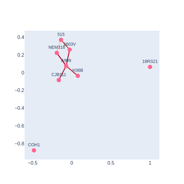
visualize_simplicial_complex(simplex_tree3,270,strains_names)
Solution

There is a 1-holes in the barcode diagram, so there is preliminary evidence that this resistome was not acquired only via vertical inheritance

By employing TDA and persistent homology, we gain a powerful lens through which to observe and understand the impact of HGT on bacterial genomes. This approach not only underscores the utility of TDA in genomic research but also highlights its potential to uncover intricate gene transfer patterns that are critical for understanding bacterial evolution and antibiotic resistance.

Key Points

Horizontal Gene Transfer (HGT) is a phenomenon where an organism transfers genetic material to another one that is not its descendant.

1-holes can detect HGT.

previous episode

Topological Data Analysis for Pangenomics

next episode

Detecting horizontal gene transfer

Overview

Introduction to Horizontal Gene Transfer

Know more: Mechanisms of HGT

Extra content

Understanding Persistent Homology in the Context of HGT:

Know more: TDA in genomics

Importing Libraries

Defining Fuctions

Case Study 1: Vertical Inheritance in a Simulated Population

Case Study 2: Introducing Horizontal Gene Transfer

Persistent Homolgy in the Streptococcus agalactiae genomes

Exercise 1(Beginner): Manipulating dataframes

Solution

Exercise 2(Beginner): Persistent homology of S. agalactiae resistome

Solution

Exercise 3(Beginner): Plot the persistent barcode of S. agalactiae resistome

Solution

Exercise 4(Intermediate): Are the S_agalaciae resistome product of vertical inheritance?

Solution

Key Points

previous episode

next episode