Persistence Simplices gives rise to Gene Families

Overview

Teaching: 30 min
Exercises: 20 min

Questions

How can I apply TDA to describe Pangenomes?

How can persistence simplices be related to gene families?

Objectives

Describe Pangenomes using Gudhi

Finding persistence families of genes

Explore the change of gene families by varying the distance parameter

Persistent approach to pangenomics

We will work with the four mini-genomes of episode Measuring Sequence Similarity. First, we need to import all the libraries that we will use.

import pandas as pd
from matplotlib import cm
import numpy as np
import gudhi
import time
import os  

Now, we need to read the mini-genomes.blast file that we produced in the episode of Measuring Sequence Similarity.

url = "https://raw.githubusercontent.com/carpentries-incubator/pangenomics/gh-pages/files/mini-genomes.blast"
blastE = pd.read_csv(url, sep='\t', names=['qseqid', 'sseqid', 'evalue'])
 

Obtain a list of the unique genes.

qseqid_unique=pd.unique(blastE['qseqid'])
sseqid_unique=pd.unique(blastE['sseqid'])
genes = pd.unique(np.append(qseqid_unique, sseqid_unique))

We have 43 unique genes, we can check it as follows.

len(genes)

Also, we will need a list of the unique genomes in our database. First, we convert to a data frame object the list of genes, then we split each gene in the genome and gen part, and finally we obtain a list of the unique genomes and save it in the object genomes.

df_genes=pd.DataFrame(genes, columns=['Genes'])
df_genome_genes=df_genes["Genes"].str.split("|", n = 1, expand = True)
df_genome_genes.columns= ["Genome", "Gen"]
genomes=pd.unique(df_genome_genes['Genome'])
genomes=list(genomes)
genomes

['2603V', '515', 'A909', 'NEM316']

To use the gudhi packages, we need a distance matrix. In this case, we will use the evalue as the measure of how similar the genes are. First, we will process the blastE data frame to a list and then we will convert it into a matrix object.

distance_list = blastE[ blastE['qseqid'].isin(genes) & blastE['sseqid'].isin(genes)]
distance_list.head()

  qseqid	              sseqid	              evalue
2603V|GBPINHCM_01420	NEM316|AOGPFIKH_01528	4.110000e-67
2603V|GBPINHCM_01420	A909|MGIDGNCP_01408	4.110000e-67
2603V|GBPINHCM_01420	515|LHMFJANI_01310	4.110000e-67
2603V|GBPINHCM_01420	2603V|GBPINHCM_01420	4.110000e-67
2603V|GBPINHCM_01420	A909|MGIDGNCP_01082	1.600000e+00

As we saw in episode Measuring Sequence Similarity, the BLAST E-value represents the possibility of finding a match with a similar score in a database. By default, BLAST considers a maximum score for the E-value 10, but in this case, there are hits of low quality. If two sequences are not similar or if the E-value is bigger than 10, then BLAST does not save this score. In order to have something like a distance matrix we will fill the E-value of the sequence for which we do not have a score. To do this, we will use the convention that an E-value equal to 5 is too big and that the sequences are not similar at all.

MaxDistance = 5.0000000

# reshape long to wide
matrixE = pd.pivot_table(distance_list,index = "qseqid",values = "evalue",columns = 'sseqid')
matrixE.iloc[1:5,1:5]

sseqid	2603V|GBPINHCM_00065	2603V|GBPINHCM_00097	2603V|GBPINHCM_00348	2603V|GBPINHCM_00401
qseqid				
2603V|GBPINHCM_00065	1.240000e-174	NaN	NaN	NaN
2603V|GBPINHCM_00097	NaN	9.580000e-100	NaN	NaN
2603V|GBPINHCM_00348	NaN	NaN	0.0	NaN
2603V|GBPINHCM_00401	NaN	NaN	NaN	2.560000e-135

matrixE2=matrixE.fillna(MaxDistance)
matrixE2.iloc[0:4,0:4]

sseqid	2603V|GBPINHCM_00065	2603V|GBPINHCM_00097	2603V|GBPINHCM_00348	2603V|GBPINHCM_00401
qseqid				
2603V|GBPINHCM_00065	1.240000e-174	5.000000e+00	5.0	5.000000e+00
2603V|GBPINHCM_00097	5.000000e+00	9.580000e-100	5.0	5.000000e+00
2603V|GBPINHCM_00348	5.000000e+00	5.000000e+00	0.0	5.000000e+00
2603V|GBPINHCM_00401	5.000000e+00	5.000000e+00	5.0	2.560000e-135

We need to have an object with the names of the columns of the matrix that we will use later.

name_columns = matrixE2.columns
name_columns

Index(['2603V|GBPINHCM_00065', '2603V|GBPINHCM_00097', '2603V|GBPINHCM_00348',
       '2603V|GBPINHCM_00401', '2603V|GBPINHCM_00554', '2603V|GBPINHCM_00748',
       '2603V|GBPINHCM_00815', '2603V|GBPINHCM_01042', '2603V|GBPINHCM_01226',
       '2603V|GBPINHCM_01231', '2603V|GBPINHCM_01420', '515|LHMFJANI_00064',
 ...,
       'NEM316|AOGPFIKH_01341', 'NEM316|AOGPFIKH_01415',
       'NEM316|AOGPFIKH_01528', 'NEM316|AOGPFIKH_01842'],
      dtype='object', name='sseqid')

Finally, we need the distance matrix as a numpy array.

DistanceMatrix = matrixE2.to_numpy()
DistanceMatrix

array([[1.24e-174, 5.00e+000, 5.00e+000, ..., 5.00e+000, 5.00e+000,
        5.00e+000],
       [5.00e+000, 9.58e-100, 5.00e+000, ..., 5.00e+000, 5.00e+000,
        5.00e+000],
       [5.00e+000, 5.00e+000, 0.00e+000, ..., 5.00e+000, 5.00e+000,
        5.00e+000]

Now, we want to construct the Vietoris-Rips complex associated with the genes with respect to the distance matrix that we obtained. In the episode Introduction Topological Data Analysis we saw that to construct the Vietoris-Rips complex we need to define a distance parameter or threshold, so the points within a distance less than or equal to the threshold get connected in the complex. The threshold is defined by the argument max_edge_length, and we will use here the value 2.

max_edge_length = 2
# Rips complex with the distance matrix
start_time = time.time()
ripsComplex = gudhi.RipsComplex(
    distance_matrix = DistanceMatrix, 
    max_edge_length = max_edge_length
)
print("The Rips complex was created in %s" % (time.time() - start_time) )

The Rips complex was created in 0.00029540061950683594

Discussion: Changing the maximum dimension of the edges

To create the Rips Complex, we fixed that the maximum edge length was 2. What happens if we use a different parameter?
For example, if we use max_edge_lenght=1. Do you expect to have more simplices? Why?

Solution

If we use a different max_edge_length we will obtain a differente filtration with less or more simplices. In the case of max_edge_lenght=1 we will have less simplices because we stop the creation of simplices when the radius of the balls around the simplices are 1.

As we see in the previous episodes, we now need a filtration. We will use the gudhi function create_simplex_tree to obtain the filtration associated with the Rips complex. We need to specify the argument max_dimension, this argument is the maximum dimension of the simplicial complex that we will obtain. If it is for example 4, this means that we will obtain gene families with at most 4 genes. In this example, we will use 8 as the maximum dimension so we can have families with at most 2 genes from each genome or 8 different genes.

Note

For complete genomes, the maximum dimension of the simplicial complex needs to be carefully chosen because the computation in Python is demanding in terms of system resources. For example, with 4 complete genomes the maximum dimension that we can compute is 5.

start_time = time.time()
simplexTree = ripsComplex.create_simplex_tree(
    max_dimension = 8)
print("The filtration of the Rips complex was created in %s" % (time.time() - start_time))

The filtration of the Rips complex was created in 0.001073598861694336

With the persistence() function, we will obtain the persistence of each simplicial complex.

start_time = time.time()
persistence = simplexTree.persistence()  
print("The persistente diagram of the Rips complex was created in %s" % (time.time() - start_time))

The persistente diagram of the Rips complex was created in 0.006387233734130859

We can print the birth time of the simplices. If we check the output of the following, we can see the simplices with how many vertices they have and with the birth time of each.

result_str = 'Rips complex of dimension ' + repr(simplexTree.dimension())
print(result_str)
fmt = '%s -> %.2f'
for filtered_value in simplexTree.get_filtration():
    print(tuple(filtered_value))

Rips complex of dimension 7
([0], 0.0)
([1], 0.0)
([2], 0.0)
([3], 0.0)
([4], 0.0)
([5], 0.0)
([6], 0.0)
([7], 0.0)
...

simplexTree.dimension(), simplexTree.num_vertices(), simplexTree.num_simplices()

(7, 43, 467)

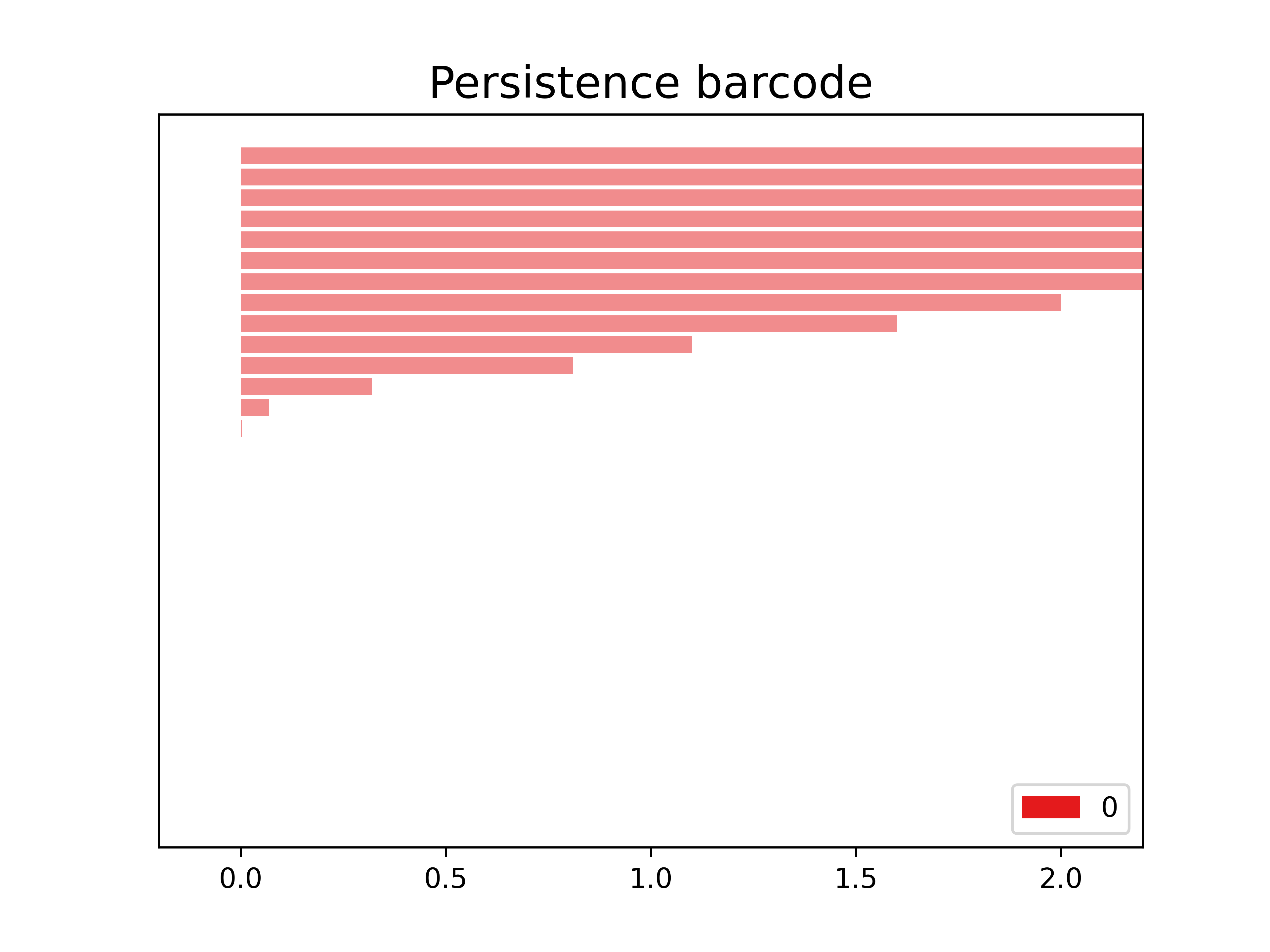
The following is the barcode of the filtration that we created. We observe in this case that we only have objects in dimension 0.

start_time = time.time()
gudhi.plot_persistence_barcode(
    persistence = persistence, 
    alpha = 0.5,
    colormap = cm.Set2.colors
)
print("Bar code diagram was created in %s" % (time.time() - start_time))

Bar code diagram was created in 0.05829215049743652

The following function allows us to obtain the dimension of the simplices.

def dimension(list):
    return (len(list[0])-1, list[1])

We filter according to the dimension function: it orders the simplices from largest dimension to smallest and then from longest birth time to smallest.

all_simplex_sorted_dim_1 = sorted(simplexTree.get_filtration(), key = dimension, reverse = True)
all_simplex_sorted_dim_1 

[([4, 9, 15, 18, 25, 30, 37, 39], 0.014),
 ([4, 9, 15, 18, 25, 30, 37], 0.014),
 ([4, 9, 15, 18, 25, 30, 39], 0.014),
 ([4, 9, 15, 18, 25, 37, 39], 0.014),
...
 ([35], 0.0),
 ([36], 0.0),
 ([37], 0.0),
 ([38], 0.0),
 ([39], 0.0),
 ([40], 0.0),
 ([41], 0.0),
 ([42], 0.0)]

Obtain the persistence of each simplex.

d_simplex_time = dict()
d_simplex_const = dict()
names = []
for tuple_simple in all_simplex_sorted_dim_1:
    list_aux = []
    if len(tuple_simple[0])-1 == simplexTree.dimension(): 
        t_birth = tuple_simple[1]
        t_death = max_edge_length
        d_simplex_time[tuple(tuple_simple[0])] = (t_birth,t_death)
        list_aux = tuple([name_columns[tuple_simple[0][i]] for i in range(len(tuple_simple[0]))])
        d_simplex_const[list_aux] = (t_birth,t_death)
    else:
        t_birth = tuple_simple[1] 
        t_death = max_edge_length
        for simplex in d_simplex_time.keys():
            if set(tuple_simple[0]).issubset(set(simplex)):
                t_death = d_simplex_time[simplex][0] 
        d_simplex_time[tuple(tuple_simple[0])] = (t_birth,t_death)
        list_aux = tuple([name_columns[tuple_simple[0][i]] for i in range(len(tuple_simple[0]))])
        d_simplex_const[list_aux] = (t_birth,t_death) 

We can save the name of the simplices, i.e. the keys in the object d_simplex_const, in a list called simplices.

simplices = list()
simplices = list(d_simplex_const.keys())

Now, we want an object with the information on how many genes of each genome are in each family.

bool_gen = dict()
genes_contains = dict()
num_new_columns = len(genomes)
for simplex in simplices:
    genes_contains = dict()
    genes_contains = {'2603V': 0, '515': 0, 'A909': 0, 'NEM316': 0}
    for i in range(len(simplex)):
        for genoma in genomes:
            if genoma in simplex[i]:
                genes_contains[genoma] = genes_contains[genoma] +1
    for gen in genomes:
        if gen not in genes_contains.keys():
            genes_contains[gen] = 0
    bool_gen[simplex] = genes_contains
bool_gen

The bool_gen numbers looks like:

{('2603V|GBPINHCM_00554',
  '2603V|GBPINHCM_01231',
  '515|LHMFJANI_00548',
  '515|LHMFJANI_01178',
  'A909|MGIDGNCP_00580',
  'A909|MGIDGNCP_01268',
  'NEM316|AOGPFIKH_00621',
  'NEM316|AOGPFIKH_01341'): {'2603V': 2, '515': 2, 'A909': 2, 'NEM316': 2},
 ('2603V|GBPINHCM_00554',
  '2603V|GBPINHCM_01231',
  '515|LHMFJANI_00548',
  '515|LHMFJANI_01178',
  'A909|MGIDGNCP_00580',
  'A909|MGIDGNCP_01268',
  'NEM316|AOGPFIKH_00621'): {'2603V': 2, '515': 2, 'A909': 2, 'NEM316': 1},
...
('NEM316|AOGPFIKH_00855',): {'2603V': 0, '515': 0, 'A909': 0, 'NEM316': 1},
 ('NEM316|AOGPFIKH_01341',): {'2603V': 0, '515': 0, 'A909': 0, 'NEM316': 1},
 ('NEM316|AOGPFIKH_01415',): {'2603V': 0, '515': 0, 'A909': 0, 'NEM316': 1},
 ('NEM316|AOGPFIKH_01528',): {'2603V': 0, '515': 0, 'A909': 0, 'NEM316': 1},
 ('NEM316|AOGPFIKH_01842',): {'2603V': 0, '515': 0, 'A909': 0, 'NEM316': 1}}

How can we read the object bool_gen?

We have a dictionary of dictionaries. Every key in the dictionary is a family and in the values, we have how many genes are from each genome in each family.

Now, we want to obtain a dataframe with information on the time of births, death, and persistence of every simplex (i.e. every family). First, we will obtain this information from our object d_simplex_time and we will save it in tree lists.

births = []
deaths = []
persistent_times = []
for values in d_simplex_time.values():
    births.append(values[0])
    deaths.append(values[1])
    persistent_times.append(values[1]-values[0])

Now that we have the information we will save it in the dataframe simplex_list

data = {
    't_birth': births,
    't_death': deaths,
    'persistence': persistent_times
}
simplex_list = pd.DataFrame(index = simplices, data = data)
simplex_list.head(4)

	t_birth	t_death	persistence
(2603V|GBPINHCM_00554, 2603V|GBPINHCM_01231, 515|LHMFJANI_00548, 515|LHMFJANI_01178, A909|MGIDGNCP_00580, A909|MGIDGNCP_01268, NEM316|AOGPFIKH_00621, NEM316|AOGPFIKH_01341)	0.014	2.000	1.986
(2603V|GBPINHCM_00554, 2603V|GBPINHCM_01231, 515|LHMFJANI_00548, 515|LHMFJANI_01178, A909|MGIDGNCP_00580, A909|MGIDGNCP_01268, NEM316|AOGPFIKH_00621)	0.014	0.014	0.000
(2603V|GBPINHCM_00554, 2603V|GBPINHCM_01231, 515|LHMFJANI_00548, 515|LHMFJANI_01178, A909|MGIDGNCP_00580, A909|MGIDGNCP_01268, NEM316|AOGPFIKH_01341)	0.014	0.014	0.000
(2603V|GBPINHCM_00554, 2603V|GBPINHCM_01231, 515|LHMFJANI_00548, 515|LHMFJANI_01178, A909|MGIDGNCP_00580, NEM316|AOGPFIKH_00621, NEM316|AOGPFIKH_01341)	0.014	0.014	0.000

Finally, we want the data frame with complete information, so we will concatenate the objects simplex_list and bool_gen in a convenient way.

aux_simplex_list = simplex_list
for gen in genomes:
    data = dict()
    dataFrame_aux = []
    for simplex in simplices:
        data[simplex] = bool_gen[simplex][gen]
    dataFrame_aux = pd.DataFrame.from_dict(data, orient='index', columns = [str(gen)])
    aux_simplex_list=pd.concat([aux_simplex_list, dataFrame_aux], axis = 1)
aux_simplex_list.head(4)

	t_birth	t_death	persistence	2603V	515	A909	NEM316
(2603V|GBPINHCM_00554, 2603V|GBPINHCM_01231, 515|LHMFJANI_00548, 515|LHMFJANI_01178, A909|MGIDGNCP_00580, A909|MGIDGNCP_01268, NEM316|AOGPFIKH_00621, NEM316|AOGPFIKH_01341)	0.014	2.000	1.986	2	2	2	2
(2603V|GBPINHCM_00554, 2603V|GBPINHCM_01231, 515|LHMFJANI_00548, 515|LHMFJANI_01178, A909|MGIDGNCP_00580, A909|MGIDGNCP_01268, NEM316|AOGPFIKH_00621)	0.014	0.014	0.000	2	2	2	1
(2603V|GBPINHCM_00554, 2603V|GBPINHCM_01231, 515|LHMFJANI_00548, 515|LHMFJANI_01178, A909|MGIDGNCP_00580, A909|MGIDGNCP_01268, NEM316|AOGPFIKH_01341)	0.014	0.014	0.000	2	2	2	1
(2603V|GBPINHCM_00554, 2603V|GBPINHCM_01231, 515|LHMFJANI_00548, 515|LHMFJANI_01178, A909|MGIDGNCP_00580, NEM316|AOGPFIKH_00621, NEM316|AOGPFIKH_01341)	0.014	0.014	0.000	2	2	1	2

In this data frame, we can see the history of the formation of families (simplices) at the different birth and death times. If we filter at t_death=2we can see only the families that we remain with in the end.

Exercise 1(Beginner): Partitioning the pangenome

Filter the table by t_death=2, at this point in the filtration, which families are in each partition Core, Shell and Cloud? How many of these are single-copy core families?

Solution

We can filter as follows:

aux_simplex_list[aux_simplex_list['t_death']==2]

	t_birth	t_death	persistence	2603V	515	A909	NEM316
(2603V|GBPINHCM_00554, 2603V|GBPINHCM_01231, 515|LHMFJANI_00548, 515|LHMFJANI_01178, A909|MGIDGNCP_00580, A909|MGIDGNCP_01268, NEM316|AOGPFIKH_00621, NEM316|AOGPFIKH_01341)	1.400000e-02	2.0	1.986	2	2	2	2
(2603V|GBPINHCM_00401, 515|LHMFJANI_00394, 515|LHMFJANI_01625, A909|MGIDGNCP_00405, NEM316|AOGPFIKH_00403, NEM316|AOGPFIKH_01842)	1.300000e+00	2.0	0.700	1	2	1	2
(2603V|GBPINHCM_01042, 2603V|GBPINHCM_01420, 515|LHMFJANI_01310, A909|MGIDGNCP_01408, NEM316|AOGPFIKH_01528)	1.600000e+00	2.0	0.400	2	1	1	1
(2603V|GBPINHCM_00065, 515|LHMFJANI_00064, A909|MGIDGNCP_00064, A909|MGIDGNCP_00627, NEM316|AOGPFIKH_00065)	8.600000e-02	2.0	1.914	1	1	2	1
(2603V|GBPINHCM_00348, 515|LHMFJANI_00342, A909|MGIDGNCP_00352, NEM316|AOGPFIKH_00350, NEM316|AOGPFIKH_01341)	3.000000e-03	2.0	1.997	1	1	1	2
(2603V|GBPINHCM_01042, A909|MGIDGNCP_01082, A909|MGIDGNCP_01408, NEM316|AOGPFIKH_01528)	1.600000e+00	2.0	0.400	1	0	2	1
(2603V|GBPINHCM_00748, 515|LHMFJANI_00064, A909|MGIDGNCP_00064, NEM316|AOGPFIKH_00065)	8.300000e-01	2.0	1.170	1	1	1	1
(2603V|GBPINHCM_00097, 515|LHMFJANI_00097, A909|MGIDGNCP_00096, NEM316|AOGPFIKH_00098)	9.580000e-100	2.0	2.000	1	1	1	1
(2603V|GBPINHCM_00815, 515|LHMFJANI_00781, A909|MGIDGNCP_00877, NEM316|AOGPFIKH_00855)	0.000000e+00	2.0	2.000	1	1	1	1
(2603V|GBPINHCM_00748, 2603V|GBPINHCM_01042, A909|MGIDGNCP_01082)	2.000000e+00	2.0	0.000	2	0	1	0
(2603V|GBPINHCM_00748, 2603V|GBPINHCM_01042)	2.000000e+00	2.0	0.000	2	0	0	0
(2603V|GBPINHCM_00748, A909|MGIDGNCP_01082)	2.000000e+00	2.0	0.000	1	0	1	0
(515|LHMFJANI_01625, A909|MGIDGNCP_01221)	1.100000e+00	2.0	0.900	0	1	1	0
(515|LHMFJANI_01130, A909|MGIDGNCP_01221)	1.310000e-85	2.0	2.000	0	1	1	0
(A909|MGIDGNCP_01343, NEM316|AOGPFIKH_01415)	7.890000e-143	2.0	2.000	0	0	1	1
(2603V|GBPINHCM_01226,)	0.000000e+00	2.0	2.000	1	0	0	0

Partition	Num. of Families
Core	8
Shell	6
Cloud	2

Single-copy core families: 3

Excercise 2(Beginner): Looking for functional families

In the episode Measuring Sequence Similarity we saw that the genes 2603V|GBPINHCM_01420, 515|LHMFJANI_01310, A909|MGIDGNCP_01408, and NEM316|AOGPFIKH_01528 make the functional family 30S ribosomal protein. Look for these genes in the aux_simplex_list. Are they in the same family? Are there other genes in this family?

Solution

Yes, they are in the same family, but there is one more gene in this family, the gene 2603V|GBPINHCM_01042.

Exercise 3(Intermediate): Changing the dimension of the simplices

When we create the object simplexTree we define that the maximum dimension of the simplices was 8. Change this parameter to 3.
With the new parameter, how many simplices do you obtain? And edges? If you run all the code with this new parameter and filter again by t_death = 2, what happens with the partitions? How many families do you have?
Solution
start_time = time.time()
simplexTree = ripsComplex.create_simplex_tree(
   max_dimension = 3)
persistence = simplexTree.persistence()
simplexTree.dimension(), simplexTree.num_vertices(), simplexTree.num_simplices()
(3, 43, 364)
Now we have less simplices, we have 364 simplices.

When we filter by t_death = 2, we obtain 111 families because some families share genes.

Key Points

Pangenomes can be described using TDA

Persistence simplices are related to the gene families of a Pangenome

Persistence simplices can be used to find some funtional families

previous episode

Topological Data Analysis for Pangenomics

next episode

Persistence Simplices gives rise to Gene Families

Overview

Persistent approach to pangenomics

Discussion: Changing the maximum dimension of the edges

Solution

Note

Exercise 1(Beginner): Partitioning the pangenome

Solution

Excercise 2(Beginner): Looking for functional families

Solution

Exercise 3(Intermediate): Changing the dimension of the simplices

Solution

Key Points

previous episode

next episode