Survival Analysis

Estimated time: 12 minutes

Overview

Questions

• What are survival models and how do they handle censored time-to-event data?
• How can Bayesian survival models be implemented and interpreted using Stan?

Objectives

• Understand survival functions, hazard functions, and censoring in survival data.
• Learn to implement and compare Weibull and Cox proportional hazards models using Stan.
• Extend survival models with hierarchical structures and evaluate model results.

Survival (or time-to-event) data arise when the outcome of interest is the time until some event occurs, such as device failure, disease onset or death. A key difference to ordinary regression settings is that time-to-event data are commonly censored, meaning that for some data points the event has not occurred by the end of the observation period. This may happen because the study ends before the event occurs, a participant leaves the study, or the event is otherwise not observed during follow-up. This implies that the exact event time is unknown and analyses must use techniques that account for both observed event times and censored observations.

Callout

In this episode, we will exclusively analyze right-censored data, where each individual is followed until either the event occurs or the observation period ends. For censored individuals, the event time is only known to be longer than the observed follow-up time. This is the most common type of censoring, but there are two other censoring mechanisms are sometimes encountered. In left censoring, the event occurs before observation begins, so the event time is only known to be earlier than a given time point. Interval censoring means a situation where the event occurs between two observation times, but the exact timing is unknown.

Before we start building survival models in Stan, we need to first get familiar with some mathematical concepts important in survival analysis.

For each individual, we observe a follow-up time \[ Y_i=\min(T_i,C_i), \]

where \(T_i\) is the true event time and \(C_i\) is the censoring time. We also observe an indicator variable that records whether the event occurred during follow-up. This indicator is usually defined as

\[ \delta_i = \begin{cases} 1, & \text{if } T_i \leq C_i \quad \text{(event observed)},\\ 0, & \text{if } T_i > C_i \quad \text{(right censored)}. \end{cases} \]

The two functions central to specifying common survival models are the survival function \(S(t) = P(T > t)\) and the hazard function \(h(t)\). The former gives the probability of surviving beyond time \(t\), whereas the latter describes the instantaneous event rate at time \(t\) among individuals who have not experienced the event before \(t\). Formally the hazard is defined as \[h(t) = \lim_{dt \to 0} \dfrac{P(t \le T < t + dt \mid T \ge t)}{dt}. \] These two functions are linked through the identity \(S(t) = \exp\{-H(t)\},\) where \(H(t)\) is the cumulative hazard, representing the accumulated hazard up to time \(t\), \(H(t) = \int_0^t h(u)\,du\).

While a wealth of various tools for survival analysis have been presented, including modern machine learning approaches, in this episode, we will focus on two relatively standard models: the parametric Weibull model and the semiparametric Cox proportional hazards model. Both of these models use the multiplicative form \(h(t \mid x) = h_0(t)\,\exp(x^\top \beta),\) where \(h_0(t)\) is the baseline hazard describing hazard evolution when covariates equal zero.

A key distinction between the two models is that the Weibull model uses an explicit functional form for the baseline hazard (and simultaneously for the event times), while in the Cox model this is left unspecified. The Weibull model gains statistical strength from this assumed functional form. However, a mismatch between the assumption and data can lead to a poor model fit. The Cox model, on the other hand, can be more robust when the baseline hazard shape is unknown. Both approaches enable assessment of covariate effects on survival. The Weibull model provides survival predictions directly through its assumed distribution, whereas Cox models require an estimate of the baseline hazard to obtain absolute survival predictions.

Censored observations contribute information through the survival function, because although the exact event time is unknown, we know that the event has not occurred before the observed follow-up time. In other words, the contribution of a censored observation is the probability that the event time exceeds the censoring threshold, namely \(1-F_T(t^{cens})\), where \(F_T(t)=\text{Pr}(T<t)\) is the cumulative distribution function of survival time.

The survival models introduced above can be formulated using different statistical frameworks. In this episode, we adopt a Bayesian approach and implement survival models using Stan. We focus on how the Bayesian framework extends survival analysis by representing model parameters through posterior distributions, allowing uncertainty in survival quantities of interest to be quantified directly.

Bayesian survival analysis

---

The survival models introduced above describe the relationship between covariates and time-to-event outcomes through quantities such as regression coefficients, hazard functions, and survival probabilities. These models can be estimated using either frequentist or Bayesian approaches. In this episode, we focus on the Bayesian formulation, where uncertainty about survival model parameters is represented through posterior distributions.

The main difference between classical and Bayesian survival analysis is how uncertainty is handled. Traditional survival models typically provide point estimates of parameters together with uncertainty measures based on large-sample approximations. In contrast, Bayesian survival models estimate a posterior distribution for each unknown parameter by combining the survival likelihood with prior distributions.

For survival models, the likelihood accounts for both observed events and censored observations. After combining this likelihood with prior information, we obtain posterior distributions for model parameters such as regression coefficients, Weibull shape parameters, and hierarchical effects.

Using Stan, we obtain samples from these posterior distributions through Markov chain Monte Carlo (MCMC) methods. These posterior draws allow us to directly calculate uncertainty for quantities of interest in survival analysis. For example, instead of estimating a single hazard ratio, we obtain its posterior distribution:

\[ HR=\exp(\beta). \]

Similarly, posterior samples can be transformed to obtain survival curves, median survival times, and predictions for new individuals while naturally propagating parameter uncertainty.

Before implementing the survival models in Stan, we first introduce the experimental dataset that will be used throughout this episode. This dataset provides time-to-event outcomes and relevant covariates, allowing us to apply the Bayesian survival framework developed above in a practical setting.

Survival data

---

To demonstrate survival analysis in Stan, we will analyze a real-world biological dataset containing gut microbiome profiles from laboratory-grown mice (ref?). The aim is to investigate whether the abundance of specific bacterial genera measured in stool samples is associated with the time until Type 1 Diabetes (T1D) onset.

For each mouse, the dataset contains:

• the observed follow-up time (Event_time), corresponding to the survival observation \((Y_i=\min(T_i,C_i))\),
• an event indicator (Event), where 1 denotes diabetes onset during follow-up and 0 indicates right censoring, and
• measurements of bacterial abundances for 48 microbial genera, which are used as covariates in the survival models.

The dataset is provided as a TreeSummarizedExperiment object in the lesson repository. We use the mia package for microbiome data manipulation and analysis, and to work with microbiome assays stored in the TreeSummarizedExperiment format.

Before fitting survival models, we preprocess the microbial abundance data using a standard workflow:

1. Relative abundance transformation: Raw sequencing counts are converted into relative abundances to account for differences in sequencing depth between samples.

2. Prevalence filtering: Microbial genera that are rarely observed across samples are removed to reduce sparsity and improve the reliability of abundance estimates. A genus is considered present when its relative abundance exceeds a predefined detection threshold, and only genera observed in a sufficient fraction of samples are retained.

3. Logarithmic transformation: Since microbial abundance data are highly skewed and may contain zero values, the retained microbial abundances are log-transformed using a small pseudocount to stabilize variance and improve numerical behavior.

4. Standardization: Continuous microbial abundance covariates are standardized to have mean 0 and standard deviation 1. This improves computational stability during Hamiltonian Monte Carlo sampling in Stan. Additionally, hazard ratios can be interpreted as the change in hazard associated with a one standard deviation increase in log-transformed microbial abundance.

The following code loads the dataset, performs the pre-processing steps, and prepares the data structure required for survival model implementation in Stan.

R

# Load required libraries for data processing and handling
library(tidyverse)
library(cmdstanr)
library(posterior) 
library(survival)
library(TreeSummarizedExperiment)
library(survminer)
# library(mia)

R

# Load TSE
tse <- readRDS(file.path("data", "survival_tse.rds"))


# Relative abundance transformation
counts <- SummarizedExperiment::assay(tse, "counts")

sample_totals <- colSums(counts)

if (any(sample_totals == 0)) {
  stop("At least one sample has a total count of zero.")
}

rel <- sweep(
  counts,
  MARGIN = 2,
  STATS = sample_totals,
  FUN = "/"
)


# Extract relative abundance matrix
rel <- assay(tse, "relabundance")

ERROR

Error in `assay()`:
! 'assay(<TreeSummarizedExperiment>, i="character", ...)' invalid subscript 'i'
'relabundance' not in names(assays(<TreeSummarizedExperiment>))

R

# Prevalence filtering
# A genus is considered present if relative abundance >= 0.1%
REL_PRES_MIN <- 1e-3

# Retain genera present in at least 30% of samples
PREV_MIN <- 0.30

genus_prevalence <- rowMeans(rel >= REL_PRES_MIN)

selected_microbes <- names(
  genus_prevalence[genus_prevalence >= PREV_MIN]
)

length(selected_microbes)

OUTPUT

[1] 28

R

# Log transform selected microbial abundances
log_abund <- log(
  rel[selected_microbes, , drop = FALSE] + 1e-6
)

df <- as.data.frame(t(log_abund))

# Outcomes
df$Event <- sample_data$Event

ERROR

Error:
! object 'sample_data' not found

R

df$Event_time <- sample_data$Event_time

ERROR

Error:
! object 'sample_data' not found

R

# Build design matrix (scaled)
X <- scale(
  as.matrix(df[, selected_microbes, drop = FALSE])
)

K <- ncol(X)


# Analysis data frame
analysis_df <- data.frame(
  time  = as.numeric(df$Event_time),
  event = as.integer(df$Event),
  X,
  check.names = FALSE
)

ERROR

Error in `data.frame()`:
! arguments imply differing number of rows: 0, 150

R

rownames(analysis_df) <- rownames(df)

ERROR

Error:
! object 'analysis_df' not found

R

# Stan data
standata <- list(
  N     = nrow(analysis_df),
  K     = K,
  time  = as.vector(analysis_df$time),
  event = as.integer(analysis_df$event),
  X     = as.matrix(
    analysis_df[, colnames(X), drop = FALSE]
  )
)

ERROR

Error in `h()`:
! error in evaluating the argument 'x' in selecting a method for function 'nrow': object 'analysis_df' not found

After prevalence filtering, the remaining microbial genera were included as covariates in the survival models. In this dataset, 28 microbial genera passed the filtering criteria.

Before fitting any survival models, it is good practice to inspect the processed dataset and verify that the survival outcomes and covariates have been prepared correctly. In particular, we check that the dataset contains both observed events and right-censored observations, and that the follow-up times and covariates have the expected structure.

R

# Inspect the structure of the analysis dataset
glimpse(analysis_df)

ERROR

Error:
! object 'analysis_df' not found

R

# Check the number of observed events and censored observations
table(analysis_df$event)

ERROR

Error:
! object 'analysis_df' not found

R

# Inspect the distribution of follow-up times
summary(analysis_df$time)

ERROR

Error in `h()`:
! error in evaluating the argument 'object' in selecting a method for function 'summary': object 'analysis_df' not found

R

# View the first observations
head(analysis_df)

ERROR

Error in `h()`:
! error in evaluating the argument 'x' in selecting a method for function 'head': object 'analysis_df' not found

Kaplan–Meier estimate

---

Before fitting parametric survival models, we first visualize the observed survival experience using the Kaplan–Meier estimator. Unlike the Weibull and Cox models introduced later, the Kaplan–Meier estimator is a non-parametric method that does not assume a specific distribution for the event times.

The Kaplan–Meier estimator provides an estimate of the survival function

\[ S(t)=P(T>t), \]

and naturally incorporates right-censored observations. Censored individuals contribute information up to their last observed follow-up time, after which their event status remains unknown.

For our dataset, the Kaplan–Meier curve represents the estimated probability that a mouse remains free of Type 1 Diabetes (T1D) as follow-up time increases. This provides an exploratory summary of the observed survival patterns before introducing model-based estimates.

R

# Kaplan-Meier estimate
km_fit <- survfit(
  Surv(time, event) ~ 1,
  data = analysis_df
)

ERROR

Error:
! object 'analysis_df' not found

R

# Plot Kaplan-Meier curve
ggsurvplot(
  km_fit,
  data = analysis_df,
  conf.int = TRUE,
  risk.table = TRUE,
  xlab = "Follow-up time (years)",
  ylab = "Probability of remaining diabetes-free",
  ggtheme = theme_bw()
)

ERROR

Error:
! object 'km_fit' not found

The Kaplan–Meier curve shows a gradual decline in diabetes-free survival over the follow-up period, with increasing uncertainty at later times due to fewer individuals remaining at risk. While this provides an overall view of survival patterns, it does not explain the factors associated with differences in event risk. Therefore, we next introduce Bayesian survival models with microbial covariates to investigate these associations.

Weibull survival model

---

The Weibull model is a parametric survival model that specifies a probability distribution for event times. In the Bayesian framework, the unknown Weibull parameters and regression coefficients are treated as uncertain quantities and estimated through their posterior distributions. The distribution has two parameters: shape \(k>0\) and scale \(\lambda>0\). A common way to include covariates in the model is to let the scale parameter depend on a linear predictor,

\[ \lambda = \exp(\beta_0 + \beta_1X_1 + \cdots + \beta_KX_K), \] where \(X_i\) are the covariate values and \(\beta_i\) are the corresponding regression coefficients. Here, the covariates enter the model through the scale parameter, corresponding to an accelerated failure time (AFT) parameterization. Since the scale parameter determines the time scale of the distribution, larger values of \(\lambda\) correspond to longer expected survival times. Consequently, positive regression coefficients increase survival time, whereas negative coefficients decrease it.

The shape parameter, on the other hand, controls how the risk evolves over time: when \(0<k<1\) the hazard decreases, with \(k=1\) it is constant, and when \(k>1\) it increases. This flexibility makes the Weibull distribution a useful starting point for modeling a wide range of survival processes.

The survival and hazard functions can be shown to take the following form (Klein and Moeschberger, 2003):

\[ S(t)=\exp\left[-\left(\frac{t}{\lambda}\right)^{k}\right], \] and \[ h(t) = \frac{k}{\lambda}\left(\frac{t}{\lambda}\right)^{k-1}. \] A convenient summary is the median survival time \[ \operatorname{med}(T)=\lambda(\log 2)^{1/k}, \] which increases linearly with \(\lambda\) and, for a fixed \(\lambda\), decreases as \(k\) increases.

Under this parameterization, increasing a covariate \(x_j\) by one unit while holding all other covariates constant results in the hazard ratio:

\[ \mathrm{HR}_j \;=\; \frac{h\!\left(t \mid x_j + 1\right)}{h\!\left(t \mid x_j\right)} \;=\; \exp\!\left(-k\,\beta_j\right). \]

Thus, under this AFT parameterization, a positive regression coefficient increases the Weibull scale parameter, leading to longer survival times and a hazard ratio smaller than one. Conversely, a negative coefficient decreases the scale parameter, resulting in shorter survival times and a hazard ratio greater than one.

Example

We now implement the Weibull survival model in Stan using the microbiome dataset introduced earlier. Our goal is to estimate the associations between microbial abundances and the time to Type 1 Diabetes onset, and to summarize these effects using posterior hazard ratios.

The Stan program for the Weibull model is shown below. The likelihood is specified using the target += notation, which directly increments the model’s log posterior density. Unlike the ~ notation, target += allows different likelihood contributions to be added explicitly for observed events and right-censored observations. This makes it well suited for survival models, where events contribute the log probability density (weibull_lpdf) and censored observations contribute the log survival probability (weibull_lccdf). The program is also written to accommodate models without covariates by allowing the number of covariates, K, to be zero.

STAN

// Weibull survival model (shape k, scale lambda), Bayesian AFT form

data {
  int<lower=1> N;                         // number of observations
  int<lower=0> K;                         // number of covariates
  vector<lower=0>[N] time;                // observed follow-up times
  array[N] int<lower=0, upper=1> event;   // 1=event, 0=right censored
  matrix[N, K] X;                         // standardized covariates
}

parameters {
  real<lower=0> k;                        // Weibull shape parameter
  real beta0;                             // intercept
  vector[K] beta;                         // regression coefficients
}

transformed parameters {
  vector<lower=0>[N] lambda;

  // AFT formulation:
  // log(lambda_i) = beta0 + X_i beta
  lambda = exp(beta0 + X * beta);
}

model {
  // Priors
  k ~ lognormal(0, 1);
  beta0 ~ normal(0, 1);
  beta ~ normal(0, 1);


  // Factorized survival likelihood
  for (i in 1:N) {

    if (event[i] == 1) {

      // Observed events:
      // contribution from Weibull density
      target += weibull_lpdf(time[i] | k, lambda[i]);

    } else {

      // Right-censored observations:
      // contribution from survival function S(t)
      target += weibull_lccdf(time[i] | k, lambda[i]);

    }
  }
}


generated quantities {

  vector[N] t_median;

  for (i in 1:N) {
    t_median[i] = lambda[i] * pow(log(2), 1.0/k);
  }
}

After fitting the Weibull model, we transform posterior draws of the regression coefficients and the Weibull shape parameter to obtain posterior distributions of hazard ratios:

\[ HR_j = \exp(-k\beta_j). \]

Because Bayesian inference provides samples from the posterior distribution, uncertainty in hazard ratios can be obtained directly by applying this transformation to every posterior draw. We summarize each hazard ratio using its posterior median and 95% credible interval.

The resulting posterior summaries are visualized using a forest plot.

R

# Fit Weibull model
fit <- weibull_model$sample(
  data = standata,
  seed = 2026,
  chains = 4,
  parallel_chains = 4,
  refresh         = 0,
  show_messages   = FALSE
)

ERROR

Error:
! 'data' should be a path or a named list.

R

# Extract posterior draws
draws <- posterior::as_draws_matrix(fit$draws())

ERROR

Error in `fit$draws`:
! object of type 'closure' is not subsettable

R

# Weibull shape parameter
k_draw <- draws[, "k"]

ERROR

Error:
! object 'draws' not found

R

K <- standata$K

ERROR

Error in `standata$K`:
! object of type 'closure' is not subsettable

R

covar_names <- colnames(standata$X)

ERROR

Error:
! error in evaluating the argument 'x' in selecting a method for function 'colnames': object of type 'closure' is not subsettable

R

# Calculate posterior hazard ratios
hr_mat <- do.call(rbind, lapply(seq_len(K), function(j) {

  beta_draw <- draws[, paste0("beta[", j, "]")]

  hr_draw <- exp(-k_draw * beta_draw)

  c(
    median = median(hr_draw),
    lower  = quantile(hr_draw, 0.025),
    upper  = quantile(hr_draw, 0.975)
  )
}))

ERROR

Error in `h()`:
! error in evaluating the argument 'args' in selecting a method for function 'do.call': object 'draws' not found

R

# Create summary data frame
hr_df <- as.data.frame(hr_mat)

ERROR

Error in `h()`:
! error in evaluating the argument 'x' in selecting a method for function 'as.data.frame': object 'hr_mat' not found

R

hr_df$term <- covar_names

ERROR

Error:
! object 'covar_names' not found

R

names(hr_df) <- c(
  "HR",
  "lower",
  "upper",
  "term"
)

ERROR

Error:
! object 'hr_df' not found

R

# Identify taxa where 95% credible interval excludes 1
hr_df$association <- 
  (hr_df$lower > 1) | (hr_df$upper < 1)

ERROR

Error:
! object 'hr_df' not found

R

# Order taxa
hr_df <- hr_df[order(hr_df$HR), ]

ERROR

Error:
! object 'hr_df' not found

R

hr_df$term <- factor(
  hr_df$term,
  levels = hr_df$term
)

ERROR

Error:
! object 'hr_df' not found

R

# Forest plot
ggplot(hr_df, aes(y = term, x = HR, color = association)) +
  geom_vline(
    xintercept = 1,
    linetype = "dashed",
    color = "grey70"
  ) +
  geom_pointrange(
    aes(xmin = lower, xmax = upper),
    size = 0.6
  ) +
  scale_x_continuous(
    trans = "log10"
  ) +
  scale_color_manual(
    values = c(`TRUE` = "firebrick", `FALSE` = "#2C3E50"), 
    guide = "none"
  ) +
  labs(
    title = "Posterior hazard ratios from Weibull model",
    x = "Hazard ratio (log scale, per SD increase)",
    y = NULL
  ) +
  theme_bw() +
  theme(
    panel.grid.minor = element_blank(),
    plot.title = element_text(face = "bold")
  )

ERROR

Error:
! object 'hr_df' not found

As evident from the forest plot, only a subset of the microbial genera have 95% credible intervals that exclude the reference value of 1, indicating posterior evidence of an association with the hazard of Type 1 Diabetes onset. Hazard ratios greater than 1 correspond to an increased instantaneous risk of diabetes onset, whereas hazard ratios less than 1 indicate a protective association. Because the microbial abundances were standardized before model fitting, each hazard ratio represents the change in hazard associated with a one standard deviation increase in the log-transformed abundance of the corresponding genus.

For the remaining genera, the 95% credible intervals include 1, indicating that the posterior uncertainty is consistent with both increased and decreased hazards.

Model discrimination

---

Besides estimating hazard ratios, it is useful to assess how well the fitted model discriminates between individuals with higher and lower event risk. A commonly used measure is Harrell’s concordance index (C-index), which is the proportion of comparable pairs of individuals whose predicted risks are correctly ordered.

The C-index ranges from 0 to 1, with 1 indicating perfect discrimination and 0.5 indicating performance no better than random ordering. Values below 0.5 suggest that the model predicts the risk ordering in the opposite direction. Comparable pairs are determined by the observed event times and censoring indicators.

R

library(survival)

# Posterior median coefficients
beta0_med <- median(draws[, "beta0"])

ERROR

Error in `h()`:
! error in evaluating the argument 'x' in selecting a method for function 'median': object 'draws' not found

R

beta_med <- sapply(seq_len(K), function(j)
  median(draws[, paste0("beta[", j, "]")])
)

ERROR

Error in `h()`:
! error in evaluating the argument 'x' in selecting a method for function 'median': object 'draws' not found

R

# Model score where larger values indicate better survival
risk_score <- beta0_med + as.matrix(standata$X) %*% beta_med

ERROR

Error:
! object 'beta0_med' not found

R

# Harrell's C-index
c_index <- concordance(
  Surv(standata$time, standata$event) ~ risk_score
)

ERROR

Error in `standata$time`:
! object of type 'closure' is not subsettable

R

c_index$concordance

ERROR

Error:
! object 'c_index' not found

The fitted Weibull model achieved a C-index of approximately 0.76, indicating that the model correctly ranks individuals according to their relative risk in about 76% of comparable pairs.

Although the C-index provides a quantitative measure of discrimination, it does not directly show how survival patterns differ between individuals with different predicted risks. To visualize this separation, individuals are divided into low- and high-risk groups based on the model-based risk score, and Kaplan–Meier survival curves are compared between the groups.

R

risk_score <- -(beta0_med + as.matrix(standata$X) %*% beta_med)

ERROR

Error:
! object 'beta0_med' not found

R

# Create data frame for Kaplan-Meier estimation
dat_km <- data.frame(
  time  = standata$time,
  event = standata$event,
  risk  = as.numeric(risk_score)
)

ERROR

Error in `standata$time`:
! object of type 'closure' is not subsettable

R

# Divide individuals into low- and high-risk groups
# based on the median predicted risk score
risk_cutoff <- median(dat_km$risk)

ERROR

Error in `h()`:
! error in evaluating the argument 'x' in selecting a method for function 'median': object 'dat_km' not found

R

dat_km$risk_group <- factor(
  ifelse(dat_km$risk >= risk_cutoff,
         "High risk",
         "Low risk"),
  levels = c("Low risk", "High risk")
)

ERROR

Error:
! object 'dat_km' not found

R

# Kaplan-Meier survival curves
km_fit <- survfit(
  Surv(time, event) ~ risk_group,
  data = dat_km
)

ERROR

Error:
! object 'dat_km' not found

R

# Plot survival curves
ggsurvplot(
  km_fit,
  data = dat_km,
  conf.int = TRUE,
  legend.title = "Predicted risk group",
  legend.labs = c("Low risk", "High risk"),
  xlab = "Time (years)",
  ylab = "Survival probability"
)

ERROR

Error:
! object 'km_fit' not found

The Kaplan–Meier curves provide a visual assessment of whether the predicted risk groups exhibit different survival patterns. Separation between the curves indicates that the model-based risk score captures meaningful differences in diabetes onset timing.

Challenge

Challenge

Generate posterior predictive event times using the fitted Weibull model.

Using posterior draws from the fitted model:

1. Simulate event times for a selected individual.
2. Summarize the predicted survival time using the posterior median and a 95% credible interval.

Show me the solution

Use the posterior samples of the Weibull parameters to generate predictive event times. For each posterior draw, calculate the individual-specific scale parameter:

\[ \lambda_i^{(s)} = \exp(\beta_0^{(s)} + x_i^\top\beta^{(s)}) \]

and simulate:

\[ T_i^{(s)} \sim \text{Weibull}(k^{(s)}, \lambda_i^{(s)}) \]

The simulated event times represent the posterior predictive distribution. Summarize these samples using their median and quantiles to obtain the posterior median survival time and the 95% credible interval.

Cox proportional hazards model

---

The Cox proportional hazards (PH) model is a semiparametric approach for time-to-event data in which covariates act multiplicatively on the hazard function. In the Bayesian formulation, the regression coefficients are treated as uncertain quantities and estimated through their posterior distributions, while the baseline hazard is not specified parametrically.

Let \(T\) be the event time and \(X\) denote the covariates. The hazard function is defined as

\[ h(t \mid X) = h_0(t)\exp(X^\top\beta), \]

where \(h_0(t)\) is the baseline hazard function and \(\beta\) represents the regression coefficients. Unlike the Weibull accelerated failure time (AFT) model, where covariates influence the survival time through the scale parameter, the Cox PH model directly describes how covariates modify the instantaneous event risk.

Through the cumulative baseline hazard,

\[ H_0(t)=\int_0^t h_0(u)\,du, \]

the survival function can be written as

\[ S(t \mid X)=\exp\left[-H_0(t)\exp(X^\top\beta)\right] =S_0(t)^{\exp(X^\top\beta)}. \]

This formulation shows that covariates act by scaling the cumulative hazard while leaving the baseline hazard unspecified.

The coefficients \(\beta\) are interpreted as log-hazard ratios. For a one-unit increase in covariate \(x_j\), while keeping other covariates fixed, the hazard changes by

\[ \mathrm{HR}_j= \frac{h(t \mid x_j+1)} {h(t \mid x_j)} =\exp(\beta_j). \]

Therefore, a positive coefficient gives

\[ \mathrm{HR}_j>1, \]

indicating an increased hazard, while a negative coefficient gives

\[ \mathrm{HR}_j<1, \]

indicating a protective association and reduced hazard.

Estimation of the Cox model is based on the partial likelihood, which compares the linear predictor of an individual experiencing the event with those of individuals who remain at risk at the same event time. This approach avoids specifying the baseline hazard function, making the Cox model a flexible alternative to fully parametric survival models.

The key assumption of the Cox PH model is the proportional hazards assumption, which states that hazard ratios between individuals remain constant over time. Under this assumption, the relative effect of covariates on the event risk does not change during the follow-up period.

In the Bayesian implementation, posterior samples of the regression coefficients are obtained through Markov chain Monte Carlo methods. These posterior draws allow direct uncertainty quantification for hazard ratios and other quantities of interest.

The Cox partial likelihood used in this implementation estimates regression coefficients without specifying the baseline hazard. This makes the model flexible for estimating relative effects, such as hazard ratios, but it does not directly provide absolute survival probabilities or event-time predictions.

Callout

When individual survival prediction is required, the baseline hazard can be modeled explicitly using flexible approaches such as spline-based baseline hazard models. These approaches retain the proportional hazards structure while allowing estimation of individual survival curves and posterior predictive event times.

Example

In this example, we illustrate the Cox proportional hazards model by estimating posterior hazard ratios and comparing risk groups using Kaplan–Meier curves. The model is implemented in Stan using the Cox partial likelihood formulation. Below is the Stan program for the model.

STAN

// Cox proportional hazards model, partial likelihood (PH form)
data {
  int<lower=1> N;                    // observations
  int<lower=0> K;                    // number of covariates
  vector<lower=0>[N] time;           // observed times t_i
  array[N] int<lower=0, upper=1> event; // 1=event, 0=right-censored
  matrix[N, K] X;                    // covariates (N x K, K can be 0)
}

transformed data {
  // Indices of observed events 
  int<lower=0> n_event = 0;
  array[N] int event_idx;
  for (i in 1:N) {
    if (event[i] == 1) {
      n_event += 1;
      event_idx[n_event] = i;
    }
  }
}

parameters {
  vector[K] beta;                    // log hazard ratios
}

model {
  // Weakly-informative prior
  if (K > 0) beta ~ normal(0, 1);

  // Cox partial log-likelihood
  vector[N] eta;
  if (K > 0) eta = X * beta; else eta = rep_vector(0, N);

  for (e in 1:n_event) {
    int i = event_idx[e];
    real lse = negative_infinity();   // log(0)
    for (j in 1:N) {
      if (time[j] >= time[i])         // j in risk set at t_i
      lse = log_sum_exp(lse, eta[j]);
    }
    target += eta[i] - lse;
  }
}

generated quantities {
  vector[K] HR;                        // per-covariate hazard ratios
  for (k in 1:K) HR[k] = exp(beta[k]);
}

The Cox model estimates the regression coefficients \(\beta\), which represent log-hazard ratios. Therefore, the hazard ratio for a one-unit increase in covariate \(x_j\), while holding other covariates constant, is calculated as

\[ \mathrm{HR}_j = \frac{h(t \mid x_j+1)} {h(t \mid x_j)} = \exp(\beta_j). \]

Unlike the Weibull AFT model, where the hazard ratio is obtained as \(\exp(-k\beta_j)\) because covariates act through the survival-time scale parameter, the Cox PH model directly models the effect of covariates on the hazard. Therefore, in the Cox model:

• \(\mathrm{HR}_j > 1\) indicates an increased hazard (shorter time to event),
• \(\mathrm{HR}_j < 1\) indicates a protective association (lower hazard and longer survival time).

In the Bayesian analysis, hazard ratios are calculated from posterior draws of \(\beta_j\) using \(\exp(\beta_j)\). The posterior median and the 95% credible interval (2.5%–97.5%) are then used to summarize the uncertainty of each microbial association.

Posterior draws of the regression coefficients are transformed into hazard ratios using \(\exp(\beta_j)\). For each genus, we summarize the posterior median hazard ratio and its 95% credible interval using an ordered forest plot.

R

# Fit the Cox proportional hazards model
fit <- cox_model$sample(
  data = standata,
  chains = 4,
  iter_warmup = 1000,
  iter_sampling = 3000,
  seed = 2025,
  refresh = 0,
  adapt_delta = 0.95
)

ERROR

Error:
! 'data' should be a path or a named list.

R

# Extract posterior draws
draws <- posterior::as_draws_matrix(fit$draws())

ERROR

Error in `fit$draws`:
! object of type 'closure' is not subsettable

R

K <- standata$K

ERROR

Error in `standata$K`:
! object of type 'closure' is not subsettable

R

covar_names <- colnames(standata$X)

ERROR

Error:
! error in evaluating the argument 'x' in selecting a method for function 'colnames': object of type 'closure' is not subsettable

R

# Posterior hazard ratios
hr_mat <- do.call(rbind, lapply(seq_len(K), function(j) {

  beta_draw <- draws[, paste0("beta[", j, "]")]

  hr_draw <- exp(beta_draw)

  c(
    median = median(hr_draw),
    lower  = quantile(hr_draw, 0.025),
    upper  = quantile(hr_draw, 0.975)
  )
}))

ERROR

Error in `h()`:
! error in evaluating the argument 'args' in selecting a method for function 'do.call': object 'draws' not found

R

hr_df <- as.data.frame(hr_mat)

ERROR

Error in `h()`:
! error in evaluating the argument 'x' in selecting a method for function 'as.data.frame': object 'hr_mat' not found

R

hr_df$term  <- covar_names

ERROR

Error:
! object 'covar_names' not found

R

names(hr_df) <- c(
  "HR",
  "lower",
  "upper",
  "term"
)

ERROR

Error:
! object 'hr_df' not found

R

hr_df$association <-
  (hr_df$lower > 1) | (hr_df$upper < 1)

ERROR

Error:
! object 'hr_df' not found

R

hr_df <- hr_df[order(hr_df$HR), ]

ERROR

Error:
! object 'hr_df' not found

R

hr_df$term  <- factor(
  hr_df$term ,
  levels = hr_df$term 
)

ERROR

Error:
! object 'hr_df' not found

R

# Forest plot
ggplot(hr_df, aes(y = term, x = HR, color = association)) +

  geom_vline(
    xintercept = 1,
    linetype = "dashed",
    color = "grey70"
  ) +

  geom_pointrange(
    aes(
      xmin = lower,
      xmax = upper
    ),
    size = 0.6
  ) +

  scale_x_continuous(
    trans = "log10"
  ) +

  scale_color_manual(
    values = c(
      `TRUE` = "firebrick",
      `FALSE` = "#2C3E50"
    ),
    guide = "none"
  ) +

  labs(
    title = "Cox PH hazard ratios",
    x = "Hazard ratio (log scale)",
    y = NULL
  ) +

  theme_bw() +

  theme(
    panel.grid.minor = element_blank(),
    plot.title = element_text(face = "bold")
  )

ERROR

Error:
! object 'hr_df' not found

In the Cox model, taxa with HR > 1 indicate increased diabetes onset hazard, while taxa with HR < 1 indicate protective associations. Taxa whose 95% credible intervals exclude 1 show stronger posterior evidence of an association, whereas intervals overlapping 1 indicate insufficient evidence for a directional effect.

Hazard ratios describe individual associations but do not measure overall model discrimination. Therefore, we evaluate the ability of the Cox model to rank individuals according to their event risk using Harrell’s concordance index (C-index). Harrell’s concordance index (C-index) measures how well the model ranks individuals according to their predicted event risk.

R

library(survival)

# Posterior median linear predictor
beta_med <- sapply(seq_len(K), function(j)
  median(draws[, paste0("beta[", j, "]")])
)

ERROR

Error in `h()`:
! error in evaluating the argument 'x' in selecting a method for function 'median': object 'draws' not found

R

# Cox risk score (higher = higher hazard)
risk_score <- -as.numeric(
  as.matrix(standata$X) %*% beta_med
)

ERROR

Error:
! error in evaluating the argument 'x' in selecting a method for function 'as.matrix': object of type 'closure' is not subsettable

R

# Harrell's C-index
c_index <- concordance(
  Surv(standata$time, standata$event) ~ risk_score
)

ERROR

Error in `standata$time`:
! object of type 'closure' is not subsettable

R

c_index$concordance

ERROR

Error:
! object 'c_index' not found

The fitted Cox model achieved a C-index of approximately 0.76, indicating that the model correctly ranks individuals in about 76% of comparable pairs. Values above 0.5 indicate better-than-random discrimination, with higher values representing stronger predictive ability.

To visualize the risk separation captured by the model, individuals are divided into high- and low-risk groups based on the median Cox risk score, and their Kaplan–Meier survival curves are compared.

R

# Cox linear predictor for risk grouping
km_risk_score <- as.numeric(
  as.matrix(standata$X) %*% beta_med
)

ERROR

Error:
! error in evaluating the argument 'x' in selecting a method for function 'as.matrix': object of type 'closure' is not subsettable

R

dat_km <- data.frame(
  time = standata$time,
  event = standata$event,
  risk = km_risk_score
)

ERROR

Error in `standata$time`:
! object of type 'closure' is not subsettable

R

# Median split
risk_cutoff <- median(dat_km$risk)

ERROR

Error in `h()`:
! error in evaluating the argument 'x' in selecting a method for function 'median': object 'dat_km' not found

R

dat_km$risk_group <- factor(
  ifelse(dat_km$risk >= risk_cutoff,
         "High risk",
         "Low risk"),
  levels = c("Low risk", "High risk")
)

ERROR

Error:
! object 'dat_km' not found

R

# Kaplan-Meier curves
km_fit <- survfit(
  Surv(time, event) ~ risk_group,
  data = dat_km
)

ERROR

Error:
! object 'dat_km' not found

R

ggsurvplot(
  km_fit,
  data = dat_km,
  conf.int = TRUE,
  legend.title = "Predicted risk group",
  legend.labs = c("Low risk", "High risk"),
  xlab = "Time",
  ylab = "Survival probability"
)

ERROR

Error:
! object 'km_fit' not found

The Kaplan–Meier curves show the survival patterns of the predicted risk groups. The high-risk group (larger \(x^\top\beta\)) shows lower survival probability, indicating earlier diabetes onset compared with the low-risk group. Clear separation between curves suggests that the Cox risk score captures meaningful differences in event risk.

Hierarchical survival model

---

In this final example, we consider a hierarchical extension of the Cox proportional hazards model using the cancer dataset from the survival package. In addition to patient-level covariates, patients are clustered by treatment institution, allowing institution-specific frailties to capture unexplained between-institution heterogeneity.

The hierarchical Cox model extends the standard Cox model by combining fixed effects for patient characteristics with random effects that account for variation between institutions. For patient \(i\) treated at institution \(g[i]\), the hazard is

\[ h_i(t)=h_0(t)\exp\!\left(x_i^\top\beta+u_{g[i]}\right), \qquad u_g\sim\mathcal{N}(0,\sigma_u^2), \]

where \(x_i\) is the vector of standardized baseline covariates, \(\beta\) are the fixed-effect regression coefficients, and \(u_g\) is the institution-specific frailty with variance \(\sigma_u^2\). The random effects allow each institution to have its own baseline risk after accounting for patient-level predictors.

All baseline covariates are standardized (mean 0 and standard deviation 1), so the hazard ratios correspond to a one-standard-deviation increase in each covariate.

R

# Data
data(cancer, package = "survival")

# Complete cases
cancer2 <- na.omit(cancer)

# Outcome: time and event indicator (status: 1=censored, 2=dead)
cancer2$time  <- cancer2$time
cancer2$event <- as.integer(cancer2$status == 2)

# Grouping factor: institution
cancer2$group <- factor(cancer2$inst)
G <- nlevels(cancer2$group)

# All baseline covariates
X_mm <- model.matrix(
  ~ age + sex + ph.ecog + ph.karno + pat.karno + meal.cal + wt.loss,
  data = cancer2
)[, -1, drop = FALSE]  # drop intercept

# Scale columns
X <- scale(X_mm)
K <- ncol(X)

# Analysis data frame
analysis_df_cancer <- data.frame(
  time  = cancer2$time,
  event = cancer2$event,
  group = cancer2$group,
  X,
  check.names = FALSE
)

# Stan data list for hierarchical Cox PH
standata_cancer <- list(
  N     = nrow(analysis_df_cancer),
  G     = G,
  group = as.integer(analysis_df_cancer$group),
  K     = K,
  time  = as.vector(analysis_df_cancer$time),
  event = as.integer(analysis_df_cancer$event),
  X     = as.matrix(analysis_df_cancer[, colnames(X), drop = FALSE])
)

The following Stan program implements the hierarchical Cox proportional hazards model by extending the standard Cox model with institution-specific random effects (frailties) while retaining the partial likelihood formulation.

STAN

// Stan: hierarchical Cox proportional hazards model
data {
  int<lower=1> N;                     // observations
  int<lower=1> G;                     // groups
  array[N] int<lower=1, upper=G> group;      // group index
  int<lower=0> K;                     // number of covariates
  vector<lower=0>[N] time;            // observed times t_i
  array[N] int<lower=0, upper=1> event;      // 1=event, 0=censored
  matrix[N, K] X;                     // covariates
}

transformed data {
  int<lower=0> n_event = 0;
  array[N] int event_idx;
  for (i in 1:N) {
    if (event[i] == 1) {
      n_event += 1;
      event_idx[n_event] = i;
    }
  }
}

parameters {
  vector[K] beta;                     // log hazard ratios
  vector[G] u_raw;                    // group effects
  real<lower=0> sigma_u;              // group SD
}

model {
  vector[N] eta;

  if (K > 0) beta ~ normal(0, 1);
  u_raw   ~ normal(0, 1);
  sigma_u ~ normal(0, 1);

  for (i in 1:N)
    eta[i] = (K > 0 ? X[i] * beta : 0) + sigma_u * u_raw[group[i]];

  for (e in 1:n_event) {
    int i = event_idx[e];
    real lse = negative_infinity();
    for (j in 1:N) {
      if (time[j] >= time[i])
        lse = log_sum_exp(lse, eta[j]);
    }
    target += eta[i] - lse;
  }
}

generated quantities {
  vector[K] HR;                       // hazard ratios
  real var_frailty = square(sigma_u); // between-group variance

  for (k in 1:K)
    HR[k] = exp(beta[k]);
}

The following code fits the hierarchical Cox model and extracts posterior samples for the fixed effects and institution-specific frailties. Hazard ratios are then obtained by exponentiating the posterior regression coefficients.

R

# Fit hierarchical Cox and plot Hazard Ratios
fit_cancer_cox_hier <- cox_hier_model$sample(
  data    = standata_cancer,
  chains  = 4, 
  iter_warm = 1000, 
  iter_sampling = 3000,
  seed    = 2026, 
  refresh = 0,
  adapt_delta = 0.95
)

OUTPUT

Running MCMC with 4 sequential chains...

Chain 1 finished in 47.1 seconds.
Chain 2 finished in 46.1 seconds.
Chain 3 finished in 48.2 seconds.
Chain 4 finished in 45.8 seconds.

All 4 chains finished successfully.
Mean chain execution time: 46.8 seconds.
Total execution time: 187.8 seconds.

R

# Summary: fixed effects + frailty variance
fit_cancer_cox_hier$summary(variables = c("beta","sigma_u","var_frailty","HR"))

OUTPUT

# A tibble: 16 × 10
   variable       mean  median     sd    mad       q5     q95  rhat ess_bulk
   <chr>         <dbl>   <dbl>  <dbl>  <dbl>    <dbl>   <dbl> <dbl>    <dbl>
 1 beta[1]      0.0965  0.0951 0.110  0.111  -0.0856   0.277   1.00   13115.
 2 beta[2]     -0.288  -0.287  0.0997 0.100  -0.455   -0.126   1.00   11897.
 3 beta[3]      0.583   0.583  0.171  0.169   0.302    0.867   1.00    7563.
 4 beta[4]      0.294   0.291  0.145  0.146   0.0560   0.539   1.00    8500.
 5 beta[5]     -0.180  -0.180  0.125  0.127  -0.385    0.0237  1.00   12726.
 6 beta[6]     -0.0221 -0.0207 0.112  0.112  -0.208    0.160   1.00   12382.
 7 beta[7]     -0.200  -0.199  0.104  0.103  -0.375   -0.0317  1.00   13881.
 8 sigma_u      0.282   0.274  0.153  0.151   0.0467   0.550   1.00    3491.
 9 var_frailty  0.103   0.0749 0.105  0.0770  0.00218  0.303   1.00    3491.
10 HR[1]        1.11    1.10   0.122  0.122   0.918    1.32    1.00   13115.
11 HR[2]        0.753   0.751  0.0751 0.0749  0.635    0.881   1.00   11897.
12 HR[3]        1.82    1.79   0.314  0.302   1.35     2.38    1.00    7563.
13 HR[4]        1.36    1.34   0.199  0.194   1.06     1.72    1.00    8500.
14 HR[5]        0.842   0.835  0.106  0.105   0.681    1.02    1.00   12726.
15 HR[6]        0.984   0.980  0.110  0.109   0.813    1.17    1.00   12382.
16 HR[7]        0.823   0.819  0.0855 0.0843  0.687    0.969   1.00   13881.
# ℹ 1 more variable: ess_tail <dbl>

R

# Posterior draws
draws_cancer <- posterior::as_draws_matrix(fit_cancer_cox_hier$draws())
K <- standata_cancer$K
covar_names_cancer <- colnames(standata_cancer$X)

# Cox PH hazard ratios
hr_df_cancer <- do.call(rbind, lapply(seq_len(K), function(j) {
  beta_draw <- draws_cancer[, paste0("beta[", j, "]")]

  hr_draw <- exp(beta_draw)
  data.frame(
    HR    = median(hr_draw),
    lower = unname(quantile(hr_draw, 0.025)),
    upper = unname(quantile(hr_draw, 0.975)),
    term  = covar_names_cancer[j],
    stringsAsFactors = FALSE
  )
}))

hr_df_cancer$signif <- (hr_df_cancer$lower > 1) | (hr_df_cancer$upper < 1)
hr_df_cancer <- hr_df_cancer[order(hr_df_cancer$HR), , drop = FALSE]
hr_df_cancer$term <- factor(hr_df_cancer$term, levels = hr_df_cancer$term)

ggplot(hr_df_cancer, aes(y = term, x = HR, color = signif)) +
  geom_vline(xintercept = 1, linetype = "dashed", color = "grey70") +
  geom_pointrange(aes(xmin = lower, xmax = upper), size = 0.6) +
  scale_x_continuous(trans = "log10") +
  scale_color_manual(values = c(`TRUE` = "firebrick", `FALSE` = "#2C3E50"),
                     guide = "none") +
  labs(title = "Hierarchical Cox PH hazard ratios (cancer data)",
       x = "Hazard ratio (log scale)", y = NULL) +
  theme_bw() +
  theme(
    panel.grid.minor = element_blank(),
    plot.title = element_text(face = "bold")
  )

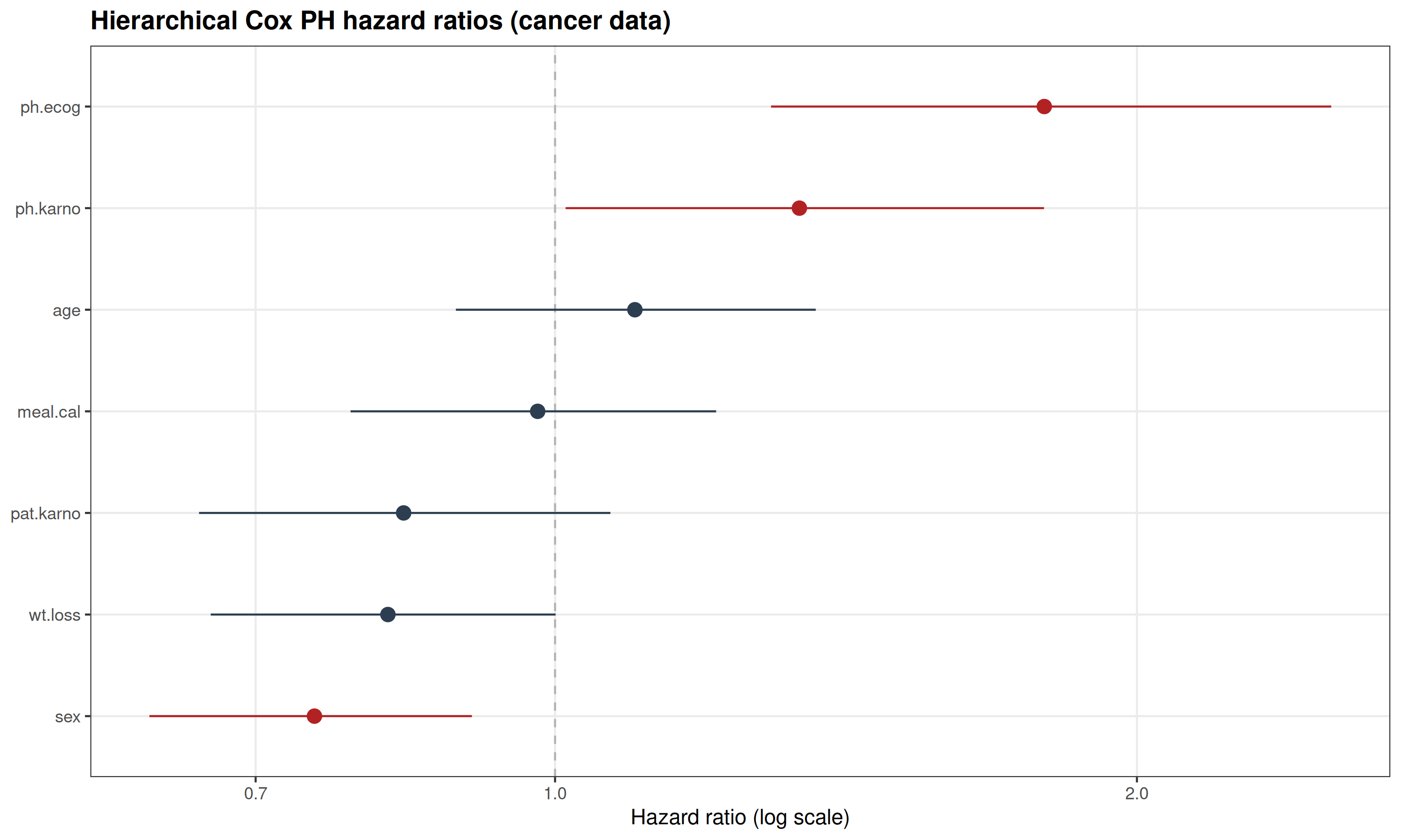
The forest plot summarizes the posterior hazard ratios for patient-level covariates after accounting for institution-specific frailty. Poorer performance status (ph.ecog and ph.karno) shows the strongest association with mortality, with hazard ratios above 1 and credible intervals excluding 1. Other covariates show weaker or more uncertain effects. The estimated frailty variance suggests some remaining between-institution heterogeneity after adjusting for patient characteristics.

we next evaluate model discrimination using Harrell’s concordance index (C-index) because these hazard ratios describe individual associations with mortality risk, they do not measure how well the model ranks patients according to their overall risk.

R

library(survival)

# Posterior median fixed effects
beta_med_cancer <- sapply(seq_len(K), function(j) {
  median(draws_cancer[, paste0("beta[", j, "]")])
})

# Patient-level risk score from fixed effects
# negative sign used so larger values correspond to better survival
risk_score_cancer <- -as.numeric(
  as.matrix(standata_cancer$X) %*% beta_med_cancer
)


# Harrell's C-index
c_index_cancer <- concordance(
  Surv(standata_cancer$time, standata_cancer$event) ~ risk_score_cancer
)

c_index_cancer$concordance

OUTPUT

[1] 0.6552442

The hierarchical Cox model achieved a C-index of approximately 0.65, indicating its ability to rank patients according to their mortality risk.

Although the C-index provides an overall measure of discrimination, it does not visualize differences in survival between risk groups. Therefore, we next compare Kaplan–Meier survival curves for patients classified into high- and low-risk groups based on the model-derived risk score.

R

# Posterior median fixed-effect coefficients
beta_med_cancer <- sapply(seq_len(K), function(j) {
  median(draws_cancer[, paste0("beta[", j, "]")])
})

# Patient-level risk score (higher = higher mortality risk)
risk_score_cancer <- as.numeric(
  as.matrix(standata_cancer$X) %*% beta_med_cancer
)

dat_km_cancer <- data.frame(
  time  = standata_cancer$time,
  event = standata_cancer$event,
  risk  = risk_score_cancer
)

# Median split of predicted risk score
risk_cutoff <- median(dat_km_cancer$risk, na.rm = TRUE)

dat_km_cancer$risk_group <- factor(
  ifelse(
    dat_km_cancer$risk >= risk_cutoff,
    "High risk",
    "Low risk"
  ),
  levels = c("Low risk", "High risk")
)

# Kaplan–Meier curves
km_fit_cancer <- survfit(
  Surv(time, event) ~ risk_group,
  data = dat_km_cancer
)

ggsurvplot(
  km_fit_cancer,
  data = dat_km_cancer,
  conf.int = TRUE,
  pval = TRUE,
  legend.title = "Model-based risk",
  legend.labs = c("Low risk", "High risk"),
  xlab = "Time",
  ylab = "Survival probability"
)

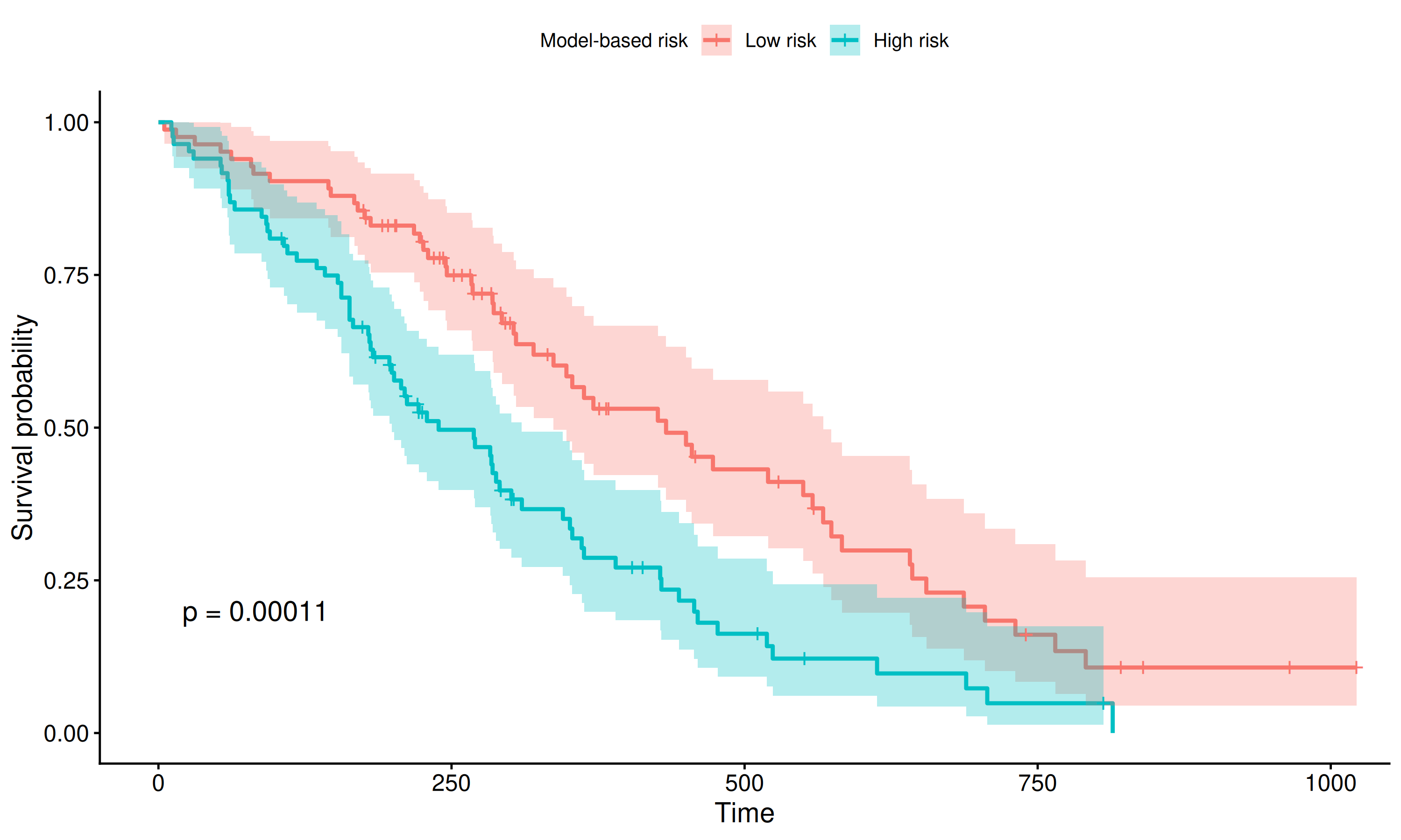
Kaplan–Meier curves by the model-based score (median split) show clear separation: the high PH risk group has lower survival, while the low-risk group remains higher. The log-rank test indicates a statistically significant difference.

Key Points

• Survival analysis models time until an event while handling censoring and aims to describe and compare time-to-event patterns across covariates or groups.

• Time-to-event outcomes can be modeled parametrically with a Weibull model that specifies survival and hazard functions or semiparametrically with a Cox proportional hazards model that leaves the baseline hazard unspecified while estimating relative risk.

• The hazard summarizes instantaneous event risk, hazard ratios compare risk between groups or covariate levels, and Kaplan–Meier curves provide a nonparametric survival estimate often shown with a log-rank test.

Challenge

Challenge

Fit a Bayesian Cox proportional hazards model with sex as the only covariate and compare the estimated hazard ratio with Kaplan–Meier survival curves.

1. Fit the Cox PH model in Stan using sex as the covariate and inspect the posterior estimates of beta and HR.
2. Transform posterior draws of beta into hazard-ratio draws and summarize the posterior median and 95% credible interval for Female vs Male.
3. Plot Kaplan–Meier curves by sex and compare the nonparametric survival patterns with the Cox model estimate.

Show me the solution

R

# Data
data(cancer, package = "survival")
cancer2 <- na.omit(cancer)

# Outcome: time and event (status: 1=censored, 2=dead)
time  <- cancer2$time
event <- as.integer(cancer2$status == 2)

# Covariate: sex (0 = Male, 1 = Female)
sex_num <- ifelse(cancer2$sex == 2, 1, 0)

# X matrix
X_sex <- matrix(sex_num, ncol = 1)
colnames(X_sex) <- "sex_female"
K <- ncol(X_sex)

standata_sex <- list(
  N    = length(time),
  K    = K,
  time = as.vector(time),
  event= as.integer(event),
  X    = X_sex
)


# Fit Cox PH -model
fit_cox_sex <- cox_model$sample(
  data = standata_sex,
  chains = 4,
  iter_warmup = 1000,
  iter_sampling = 3000,
  seed = 2025,
  refresh = 0,
  adapt_delta = 0.95
)

OUTPUT

Running MCMC with 4 sequential chains...

Chain 1 finished in 10.6 seconds.
Chain 2 finished in 10.7 seconds.
Chain 3 finished in 11.4 seconds.
Chain 4 finished in 10.4 seconds.

All 4 chains finished successfully.
Mean chain execution time: 10.8 seconds.
Total execution time: 43.5 seconds.

R

fit_cox_sex$summary("beta")

OUTPUT

# A tibble: 1 × 10
  variable   mean median    sd   mad     q5    q95  rhat ess_bulk ess_tail
  <chr>     <dbl>  <dbl> <dbl> <dbl>  <dbl>  <dbl> <dbl>    <dbl>    <dbl>
1 beta[1]  -0.462 -0.461 0.195 0.198 -0.781 -0.145  1.00    3987.    3749.

R

M_sex <- posterior::as_draws_matrix(fit_cox_sex$draws())

# log-hazard ratio Female vs Male
beta_draw  <- M_sex[, "beta[1]"]
HR_draw    <- exp(beta_draw)

HR_med     <- median(HR_draw)
HR_ci      <- quantile(HR_draw, c(0.025, 0.975))
HR_med

OUTPUT

[1] 0.6304273

R

HR_ci

OUTPUT

     2.5%     97.5%
0.4293875 0.9162222 

R

# Kaplan-Meier
cancer2$sex_factor <- factor(
  cancer2$sex,
  levels = c(1,2),
  labels = c("Male","Female")
)

sf_sex <- survfit(Surv(time, event) ~ sex_factor, data = cancer2)

ggsurvplot(
  sf_sex, data = cancer2,
  conf.int     = TRUE,
  pval         = TRUE,
  legend.title = "Sex",
  legend.labs  = c("Male", "Female"),
  xlab         = "Time", ylab = "Survival probability"
)

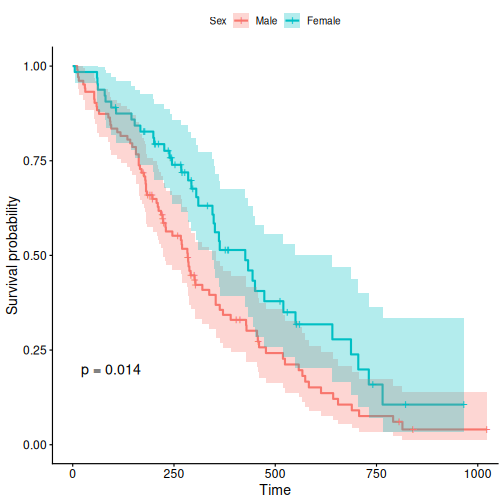
1. The posterior median hazard ratio for Female vs Male is approximately 0.63, suggesting that females have a lower estimated mortality hazard compared with males.

2. The 95% credible interval is approximately (0.43, 0.91), which is mostly below 1, indicating strong posterior support for a protective association of female sex.

3. The Kaplan–Meier curves show higher survival probabilities among females, consistent with the Cox model estimate.

The Cox model and Kaplan–Meier curves provide complementary views of survival differences: the Cox model quantifies the relative hazard, while Kaplan–Meier curves visualize the corresponding survival patterns over time.

Resources

---

• User’s guide https://mc-stan.org/docs/stan-users-guide/survival.html
• R survival package documentation: https://cran.r-project.org/package=survival
• Bürkner, P. C. (2017). brms: An R Package for Bayesian Multilevel Models Using Stan. Journal of Statistical Software, 80(1), 1–28.https://doi.org/10.18637/jss.v080.i01