Content from Short introduction to Bayesian statistics
Last updated on 2025-11-10 | Edit this page
Estimated time: 68 minutes
Overview
Questions
- How are statistical models formulated and fitted within the Bayesian framework?
Objectives
Learn to
- formulate prior, likelihood, posterior distributions.
- fit a Bayesian model with the grid approximation.
- communicate posterior information.
- work with with posterior samples.
Bayes’ formula
The starting point of Bayesian statistics is Bayes’ theorem, expressed as:
\[ p(\theta | X) = \frac{p(X | \theta) p(\theta) }{p(X)} \\ \]
When dealing with a statistical model, this theorem is used to infer the probability distribution of the model parameters \(\theta\), conditional on the available data \(X\). These probabilities are quantified by the posterior distribution \(p(\theta | X)\), which is primary the target of probabilistic modeling.
On the right-hand side of the formula, the likelihood function \(p(X | \theta)\) gives plausibility of the data given \(\theta\), and determines the impact of the data on the posterior.
A defining feature of Bayesian modeling is the second term in the numerator, the prior distribution \(p(\theta)\). The prior is used to incorporate beliefs about \(\theta\) before considering the data.
The denominator on the right-hand side \(p(X)\) is called the marginal probability, and is often practically impossible to compute. For this reason the proportional version of Bayes’ formula is typically employed:
\[ p(\theta | X) \propto p(\theta) p(X | \theta). \]
The proportional Bayes’ formula yields an unnormalized posterior distribution, which can subsequently be normalized to obtain the posterior.
Example 1: handedness
Let’s illustrate the use of the Bayes’ theorem with an example.
Assume we are trying to estimate the prevalence of left-handedness in humans, based on a sample of \(N=50\) students, out of which \(x=7\) are left-handed and 43 right-handed.
The outcome is binary and the students are assumed to be independent (e.g. no twins), so the binomial distribution is the appropriate choice for likelihood:
\[ p(X|\theta) = Bin(7 | 50, \theta). \]
Without further justification, we’ll choose \(p(\theta) = Beta(\theta |1, 10)\) as the prior distribution, so the unnormalized posterior distribution is
\[ p(\theta | X) = \text{Bin}(7 | 50, \theta) \cdot \text{Beta}(\theta | 1, 10). \]
Below, we’ll plot these functions. Likelihood (which is not a distribution!) has been normalized for better illustration.
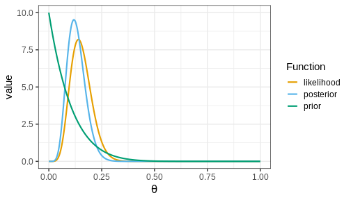
The figure shows that the majority of the mass in the posterior distribution is concentrated between 0 and 0.25. This implies that, given the available data and prior distribution, the model is fairly confident that the value of \(\theta\) is between these values. The peak of the posterior is at approximately 0.1 representing the most likely value. This aligns well with intuitive expectations about left-handedness in humans.
Actual value from a study from 1975 with 7,688 children in US grades 1-6 was 9.6%
Hardyck, C. et al. (1976), Left-handedness and cognitive deficit https://en.wikipedia.org/wiki/Handedness
Communicating posterior information
The posterior distribution \(p(\theta | X)\) contains all the information about \(\theta\) given the data, chosen model, and the prior distribution. However, understanding a distribution in itself can be challenging, especially if it is multidimensional. To effectively communicate posterior information, methods to quantify the information contained in the posterior are needed. Two commonly used types of estimates are point estimates, such as the posterior mean, mode, and variance, and posterior intervals, which provide probabilities for ranges of values.
Two specific types of posterior intervals are often of interest:
Credible intervals (CIs): These intervals leave equal posterior mass below and above them, computed as posterior quantiles. For instance, a 90% CI would span the range between the 5% and 95% quantiles.
Defined boundary intervals: Computed as the posterior mass for specific parts of the parameter space, these intervals quantify the probability for given parameter conditions. For example, we might be interested in the posterior probability that \(\theta > 0\), \(0<\theta<0.5\), or \(\theta<0\) or \(\theta > 0.5\). These probabilities can be computed by integrating the posterior over the corresponding sets.
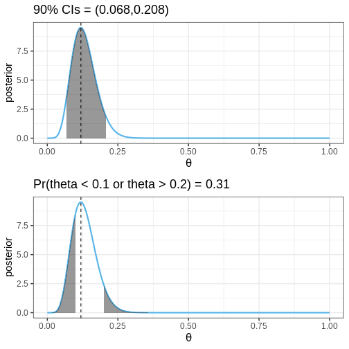
The following figures illustrate selected posterior intervals for the previous example along with the posterior mode, or maximum a posteriori (MAP) estimate.
Grid approximation
Specifying a probabilistic model can be simple, but a common bottleneck in Bayesian data analysis is model fitting. Later in the course, we will begin using Stan, a state-of-the-art method for approximating the posterior. However, we’ll begin fitting probabilistic model using the grid approximation. This approach involves computing the unnormalized posterior distribution at a grid of evenly spaced values in the parameter space and can be specified as follows:
- Define a grid of parameter values.
- Compute the prior and likelihood on the grid.
- Multiply to get the unnormalized posterior.
- Normalize.
Now, we’ll implement the grid approximation for the handedness example in R.
Example 2: handedness with grid approximation
First, we’ll load the required packages, define the data variables, and the grid of parameter values
R
# Sample size
N <- 50

# 7/50 are left-handed
x <- 7

# Define a grid of points in the interval [0, 1], with 0.01 interval
delta <- 0.01
theta_grid <- seq(from = 0, to = 1, by = delta)
Computing the values of the likelihood, prior, and unnormalized posterior is straightforward. While you can compute these using for-loops, vectorization as used below, is a more efficient approach:
R
likelihood <- dbinom(x = x, size = N, prob = theta_grid)
prior <- dbeta(theta_grid, 1, 10)
posterior <- likelihood*prior
Next, the posterior needs to be normalized.
In practice, this means dividing the values by the area under the unnormalized posterior. The area is computed with the integral \[\int_0^1 p(\theta | X)_{\text{unnormalized}} d\theta,\] which is for a grid approximated function is the sum \[\sum_{\text{grid}} p(\theta | X)_{\text{unnormalized}} \cdot \delta,\] where \(\delta\) is the grid interval.
R
# Normalize
posterior <- posterior/(sum(posterior)*delta)
# Likelihood also normalized for better visualization
likelihood <- likelihood/(sum(likelihood)*delta)
Finally, we can plot these functions
R
# Make data frame
df1 <- data.frame(theta = theta_grid, likelihood, prior, posterior)

# Wide to long format
df1_l <- df1 %>%
  gather(key = "Function", value = "value", -theta)

# Plot
p1 <- ggplot(df1_l,
       aes(x = theta, y = value, color = Function)) +
  geom_point(size = 2) +
  geom_line(linewidth = 1) +
  scale_color_grafify() +
  labs(x = expression(theta))

p1
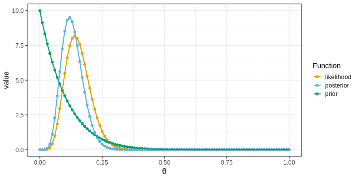
The points in the figure represent the values of the functions computed at the grid locations. The lines depict linear interpolations between these points.
Challenge
Experiment with different priors and examine their effects on the posterior. You could try, for example, different Beta distributions, the normal distribution, or the uniform distribution.
How does the shape of the prior impact the posterior?
What is the relationship between the posterior, data (likelihood) and the prior?
Grid approximation and posterior summaries
Next, we’ll learn how to compute point estimates and posterior intervals based on the approximate posterior obtained with the grid approximation.
Computing the posterior mean and variance is based on the definition of these statistics for continuous variables. The mean is defined as \[\int \theta \cdot p(\theta | X) d\theta,\] and can be computed using discrete integration: \[\sum_{\text{grid}} \theta \cdot p(\theta | X) \cdot \delta.\] Similarly, variance can be computed based on the definition \[\text{var}(\theta) = \int (\theta - \text{mean}(\theta))^2p(\theta | X)d\theta.\] Posterior mode is simply the grid value where the posterior is maximized.
In R, these statistics can be computed as follows:
R
data.frame(Estimate = c("Mode", "Mean", "Variance"),
           Value = c(df1[which.max(df1$posterior), "theta"],
                     sum(df1$theta*df1$posterior*delta),
                     sum(df1$theta^2*df1$posterior*delta) -
                       sum(df1$theta*df1$posterior*delta)^2))
OUTPUT
  Estimate       Value
1     Mode 0.120000000
2     Mean 0.131147540
3 Variance 0.001837869
Posterior intervals are also relatively easy to compute.
Finding the quantiles used to determine CIs is based on the cumulative distribution function of the posterior \(F(\theta) = \int_{\infty}^{\theta}p(y | X) dy\). The locations where the \(F(\theta) = 0.05\) and \(F(\theta) = 0.95\) define the 90% CIs.
Probabilities for certain parameter ranges are computed simply by integrating over the appropriate set, for example, \(Pr(\theta < 0.1) = \int_0^{0.1} p(\theta | X) d\theta.\)
Challenge
Compute the 90% CIs and the probability \(Pr(\theta < 0.1)\) for the handedness example.
R
# Quantiles
q5 <- theta_grid[which.max(cumsum(posterior)*delta > 0.05)]
q95 <- theta_grid[which.min(cumsum(posterior)*delta < 0.95)]

# Pr(theta < 0.1)
Pr_theta_under_0.1 <- sum(posterior[theta_grid < 0.1])*delta

print(paste0("90% CI = (", q5,",", q95,")"))
OUTPUT
[1] "90% CI = (0.07,0.21)"R
print(paste0("Pr(theta < 0.1) = ",
             round(Pr_theta_under_0.1, 5)))
OUTPUT
[1] "Pr(theta < 0.1) = 0.20659"Example 3: Gamma model with grid approximation
Let’s investigate another model and implement a grid approximation to fit it.
The gamma distribution arises, for example, in applications that model the waiting time between consecutive events. Let’s model the following data points as independent realizations from a \(\Gamma(\alpha, \beta)\) distribution with unknown shape \(\alpha\) and rate \(\beta\) parameters:
R
X <- c(0.34, 0.2, 0.22, 0.77, 0.46, 0.73, 0.24, 0.66, 0.64)
We’ll estimate \(\alpha\) and \(\beta\) using the grid approximation. Similarly as before, we’ll first need to define a grid. Since there are two parameters the parameter space is 2-dimensional and the grid needs to be defined at all pairwise combinations of the points of the individual grids.
R
delta <- 0.1
alpha_grid <- seq(from = 0.01, to = 15, by = delta)
beta_grid <- seq(from = 0.01, to = 25, by = delta)

# Get pairwise combinations
df2 <- expand.grid(alpha = alpha_grid, beta = beta_grid)
Next, we’ll compute the likelihood. As we assumed the data points to be independently generated from the gamma distribution, the likelihood is the product of the likelihoods of individual observations.
R
# Loop over all alpha, beta combinations
for(i in 1:nrow(df2)) {
  df2[i, "likelihood"] <- prod(
    dgamma(x = X,
           shape = df2[i, "alpha"],
           rate = df2[i, "beta"])
    )
}
Next, we’ll define priors for \(\alpha\) and \(\beta\). Only positive values are allowed, which should be reflected in the prior. We’ll use \(\Gamma\) priors with large variances.
Notice, that normalizing the posterior now requires integrating over both dimensions, hence the \(\delta^2\) below.
R
# Priors: alpha, beta ~ Gamma(2, .1)
df2 <- df2 %>%
mutate(prior = dgamma(x = alpha, 2, 0.1)*dgamma(x = beta, 2, 0.1))
# Posterior
df2 <- df2 %>%
mutate(posterior = prior*likelihood) %>%
mutate(posterior = posterior/(sum(posterior)*delta^2)) # Normalize
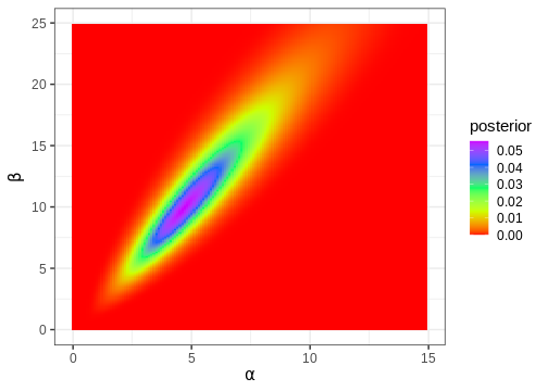
# Plot
p_joint_posterior <- df2 %>%
ggplot() +
geom_tile(aes(x = alpha, y = beta, fill = posterior)) +
scale_fill_gradientn(colours = rainbow(5)) +
labs(x = expression(alpha), y = expression(beta))
p_joint_posterior
Next, we’ll compute the posterior mode, which is a point in the 2-dimensional parameter space.
R
df2[which.max(df2$posterior), c("alpha", "beta")]
OUTPUT
      alpha beta
14898  4.71 9.91
Often, in addition to the parameters of interest, the model contains parameters we are not interested in. For instance, we might only be interested in \(\alpha\), in which case \(\beta\) would be a ‘nuisance’ parameter. Nuisance parameters are part of the full (‘joint’) posterior, but they can be discarded by integrating the joint posterior over these parameters. A posterior integrated over some parameters is called a marginal posterior.
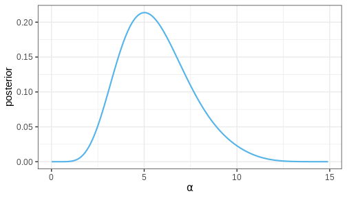
Let’s now compute the marginal posterior for \(\alpha\) by integrating over \(\beta\). Intuitively, it can be helpful to think of marginalization as a process where all of the joint posterior mass is drawn towards the \(\alpha\) axis, as if drawn by a gravitational force.
R
# Get marginal posterior for alpha
alpha_posterior <- df2 %>%
  group_by(alpha) %>%
  summarize(posterior = sum(posterior)) %>%
  mutate(posterior = posterior/(sum(posterior)*delta))

p_alpha_posterior <- alpha_posterior %>%
  ggplot() +
  geom_line(aes(x = alpha, y = posterior),
            color = posterior_color,
            linewidth = 1) +
  labs(x = expression(alpha))

p_alpha_posterior
Challenge
Does the MAP of the joint posterior of \(\theta = (\alpha, \beta)\) correspond to the MAPs of the marginal posteriors of \(\alpha\) and \(\beta\)?
The conjugate prior for the Gamma likelihood exists, which means there is a prior that causes the posterior to be of the same shape.
Working with samples
The main limitation of the grid approximation is that it becomes impractical for models with even a moderate number of parameters. The reason is that the number of computations grows as \(O \{ \Delta^p \}\) where \(\Delta\) is the number of grid points per model parameter and \(p\) the number of parameters. This quickly becomes prohibitive, and the grid approximation is seldom used in practice. The standard approach to fitting Bayesian models is to draw samples from the posterior with Markov chain Monte Carlo (MCMC) methods. These methods are the topic of a later episode but we’ll anticipate this now by studying how posterior summaries can be computed based on samples.
Example 4: handedness with samples
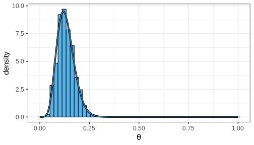
Let’s take the beta-binomial model (beta prior, binomial likelihood) of the handedness analysis as our example. It is an instance of a model for which the posterior can be computed analytically. Given a prior \(\text{Beta}(\alpha, \beta)\) and likelihood \(\text{Bin}(x | N, \theta)\), the posterior is \[p(\theta | X) = \text{Beta}(\alpha + x, \beta + N - x).\] Let’s generate \(n = 1000\) samples from this posterior using the handedness data:
R
n <- 1000
theta_samples <- rbeta(n, 1 + 7, 10 + 50 - 7)
Plotting a histogram of these samples against the grid approximation posterior displays that both are indeed approximating the same distribution
R
ggplot() +
  geom_histogram(data = theta_samples %>%
  data.frame(theta = .),
  aes(x = theta, y = after_stat(density)), bins = 50,
  fill = posterior_color, color = "black") +
    geom_line(data = df1,
            aes(x = theta, y = posterior),
            linewidth = 1.5) +
  geom_line(data = df1,
            aes(x = theta, y = posterior),
            color = posterior_color) +
  labs(x = expression(theta))
Computing posterior summaries from samples is easy. The posterior mean and variance are computed simply by taking the mean and variance of the samples, respectively. Posterior intervals are equally easy to compute: 90% CI is recovered from the appropriate quantiles and the probability of a certain parameter interval is the proportion of total samples within the interval.
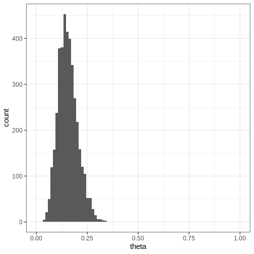
Challenge
Compute the posterior mean, variance, 90% CI and \(Pr(\theta > 0.1)\) using the generated samples.
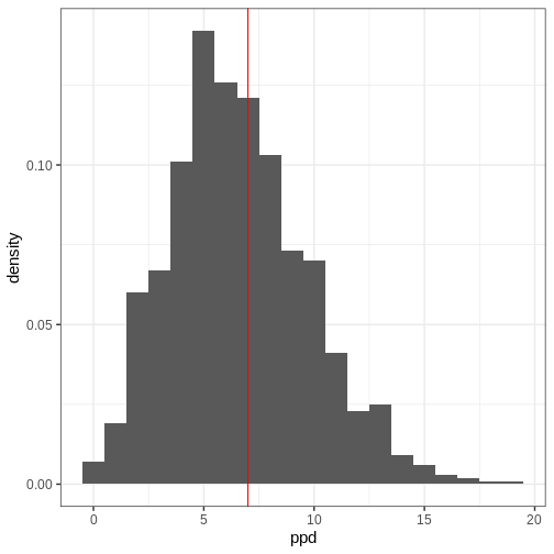
Posterior predictive distribution
Now we have learned how to fit a probabilistic model using the grid approximation and how to compute posterior summaries of the model parameters based on the fit or with posterior samples. A potentially interesting question that the posterior doesn’t directly answer is what do possible unobserved data values \(\tilde{X}\) look like, conditional on the observed values \(X\).
The unknown value can be predicted using the posterior predictive distribution \(p(\tilde{X} | X) = \int p(\tilde{X} | \theta) p(\theta | X) d\theta\). Using samples, this distribution can be sampled from by first drawing a value \(\theta^s\) from the posterior and then generating a random value from the likelihood function \(p(\tilde{X} | \theta^s)\).
A posterior predictive distribution for the beta-binomial model, using the posterior samples of the previous example can be generated as
R
ppd <- rbinom(length(theta_samples), 50, prob = theta_samples)
In other words, this is the distribution of the number of left-handed people in a yet unseen sample of 50 people. Let’s plot the histogram of these samples and compare it to the observed data (red vertical line):
R
ggplot() +
  geom_histogram(data = data.frame(ppd),
                 aes(x = ppd, y = after_stat(density)), binwidth = 1) +
  geom_vline(xintercept = 7, color = "red")
- Likelihood determines the probability of data conditional on the model parameters.
- Prior encodes beliefs about the model parameters without considering data.
- Posterior quantifies the probability of parameter values conditional on the data.
- The posterior is a compromise between the data and prior. The less data available, the greater the impact of the prior.
- The grid approximation is a method for inferring the (approximate) posterior distribution.
- Posterior information can be summarized with point estimates and posterior intervals.
- The marginal posterior is accessed by integrating over nuisance parameters.
- Usually, Bayesian models are fitted using methods that generate samples from the posterior.
Reading
- Bayesian Data Analysis (3rd ed.): Ch. 1-3
- Statistical Rethinking (2nd ed.): Ch. 1-3
- Bayes Rules!: Ch. 1-6
Content from Stan
Last updated on 2025-11-10 | Edit this page
Estimated time: 64 minutes
Overview
Questions
- How can posterior samples be generated using Stan?
Objectives
Learn how to
- implement statistical models in Stan.
- generate posterior samples with Stan.
- extract and process samples generated with Stan.
Stan is a probabilistic programming language that can be used to specify probabilistic models and to generate samples from posterior distributions.
The standard steps is using Stan is to first write the statistical model in a separate text file, then to call Stan from R (or other supported interface) which performs the sampling. Instead of having to write formulas the model can be written using built-in functions and sampling statements similar to written text. The sampling process is performed with a Markov Chain Monte Carlo (MCMC) algorithm, which we will study in a later episode. For now, however, our focus is on understanding how to execute it using Stan.
Several R packages have been built that simplify Stan usage. For example, brms allows specifying models via R’s customary formula syntax, while bayesplot provides a library of plotting functions. In this lesson, however, we will first learn using Stan from the bottom-up, by writing Stan programs, extracting the posterior samples and generating the plots ourselves. Later, in episode 7, we’ll introduce the usage of some of these additional packages.
To get started, follow the instructions provided at https://mc-stan.org/users/interfaces/ to install Stan on your local computer.
With Stan, you can fit models that have continuous parameters, but sampling from models with discrete parameters (e.g. clustering models) is not directly supported. In some cases, we can work around this by marginalizing out the discrete parameters, which makes the model fit possible in Stan. However, these workarounds are not always straightforward.
Basic program structure
A Stan program is organized into several blocks that collectively define the model. Typically, a Stan program includes at least the following blocks:
Data: This block is used to declare the input data provided to the model. It specifies the types and dimensions of the data variables incorporated into the model.
Parameters: In this block, the model parameters are declared.
Model: The likelihood and prior distributions are included here through sampling statements.
For best practices, it is recommended to specify Stan programs in separate text files with a .stan extension, which can then be called from R.
Example 1: Beta-binomial model
The following Stan program specifies the Beta-binomial model, and consists of data, parameters, and model blocks.
The data variables are the total sample size \(N\) and \(x\), the outcome of a binary variable (coin
flip, handedness etc.). The declared data type is int for
integer, and the variables have a lower bound 1 and 0 for \(N\) and \(x\), respectively. Notice that each line
ends with a semicolon.
In the parameters block we declare \(\theta\), the probability for a success. Since this parameter is a probability, it is a real number restricted between 0 and 1.
In the model block, the likelihood is specified with the sampling
statement x ~ binomial(N, theta). This line includes the
binomial distribution \(\text{Bin}(x | N,
theta)\) in the target distribution. The prior is set similarly,
and omitting the prior implies a uniform prior. Comments can be included
after two forward slashes.
STAN
  data{
    int<lower=1> N;
    int<lower=0> x;
  }

  parameters{
    real<lower=0, upper=1> theta;
  }

  model{

    // Likelihood
    x ~ binomial(N, theta);

    // Uniform prior
  }
When the Stan program has been saved we need to compile it. In R,
this is done by running the following line, where
"binomial_model.stan" is the path of the program file.
R
binomial_model <- stan_model("binomial_model.stan")
Once the program has been compiled, it can be used to generate the
posterior samples by calling the function sampling(). The
data needs to be input as a list.
R
set.seed(135)

binom_data <- list(N = 50, x = 7)

binom_samples <- sampling(object = binomial_model,
                          data = binom_data)
OUTPUT
SAMPLING FOR MODEL 'anon_model' NOW (CHAIN 1).
Chain 1:
Chain 1: Gradient evaluation took 4e-06 seconds
Chain 1: 1000 transitions using 10 leapfrog steps per transition would take 0.04 seconds.
Chain 1: Adjust your expectations accordingly!
Chain 1:
Chain 1:
Chain 1: Iteration:    1 / 2000 [  0%]  (Warmup)
Chain 1: Iteration:  200 / 2000 [ 10%]  (Warmup)
Chain 1: Iteration:  400 / 2000 [ 20%]  (Warmup)
Chain 1: Iteration:  600 / 2000 [ 30%]  (Warmup)
Chain 1: Iteration:  800 / 2000 [ 40%]  (Warmup)
Chain 1: Iteration: 1000 / 2000 [ 50%]  (Warmup)
Chain 1: Iteration: 1001 / 2000 [ 50%]  (Sampling)
Chain 1: Iteration: 1200 / 2000 [ 60%]  (Sampling)
Chain 1: Iteration: 1400 / 2000 [ 70%]  (Sampling)
Chain 1: Iteration: 1600 / 2000 [ 80%]  (Sampling)
Chain 1: Iteration: 1800 / 2000 [ 90%]  (Sampling)
Chain 1: Iteration: 2000 / 2000 [100%]  (Sampling)
Chain 1:
Chain 1:  Elapsed Time: 0.004 seconds (Warm-up)
Chain 1:                0.003 seconds (Sampling)
Chain 1:                0.007 seconds (Total)
Chain 1:

SAMPLING FOR MODEL 'anon_model' NOW (CHAIN 2).
Chain 2:
Chain 2: Gradient evaluation took 1e-06 seconds
Chain 2: 1000 transitions using 10 leapfrog steps per transition would take 0.01 seconds.
Chain 2: Adjust your expectations accordingly!
Chain 2:
Chain 2:
Chain 2: Iteration:    1 / 2000 [  0%]  (Warmup)
Chain 2: Iteration:  200 / 2000 [ 10%]  (Warmup)
Chain 2: Iteration:  400 / 2000 [ 20%]  (Warmup)
Chain 2: Iteration:  600 / 2000 [ 30%]  (Warmup)
Chain 2: Iteration:  800 / 2000 [ 40%]  (Warmup)
Chain 2: Iteration: 1000 / 2000 [ 50%]  (Warmup)
Chain 2: Iteration: 1001 / 2000 [ 50%]  (Sampling)
Chain 2: Iteration: 1200 / 2000 [ 60%]  (Sampling)
Chain 2: Iteration: 1400 / 2000 [ 70%]  (Sampling)
Chain 2: Iteration: 1600 / 2000 [ 80%]  (Sampling)
Chain 2: Iteration: 1800 / 2000 [ 90%]  (Sampling)
Chain 2: Iteration: 2000 / 2000 [100%]  (Sampling)
Chain 2:
Chain 2:  Elapsed Time: 0.004 seconds (Warm-up)
Chain 2:                0.003 seconds (Sampling)
Chain 2:                0.007 seconds (Total)
Chain 2:

SAMPLING FOR MODEL 'anon_model' NOW (CHAIN 3).
Chain 3:
Chain 3: Gradient evaluation took 1e-06 seconds
Chain 3: 1000 transitions using 10 leapfrog steps per transition would take 0.01 seconds.
Chain 3: Adjust your expectations accordingly!
Chain 3:
Chain 3:
Chain 3: Iteration:    1 / 2000 [  0%]  (Warmup)
Chain 3: Iteration:  200 / 2000 [ 10%]  (Warmup)
Chain 3: Iteration:  400 / 2000 [ 20%]  (Warmup)
Chain 3: Iteration:  600 / 2000 [ 30%]  (Warmup)
Chain 3: Iteration:  800 / 2000 [ 40%]  (Warmup)
Chain 3: Iteration: 1000 / 2000 [ 50%]  (Warmup)
Chain 3: Iteration: 1001 / 2000 [ 50%]  (Sampling)
Chain 3: Iteration: 1200 / 2000 [ 60%]  (Sampling)
Chain 3: Iteration: 1400 / 2000 [ 70%]  (Sampling)
Chain 3: Iteration: 1600 / 2000 [ 80%]  (Sampling)
Chain 3: Iteration: 1800 / 2000 [ 90%]  (Sampling)
Chain 3: Iteration: 2000 / 2000 [100%]  (Sampling)
Chain 3:
Chain 3:  Elapsed Time: 0.004 seconds (Warm-up)
Chain 3:                0.003 seconds (Sampling)
Chain 3:                0.007 seconds (Total)
Chain 3:

SAMPLING FOR MODEL 'anon_model' NOW (CHAIN 4).
Chain 4:
Chain 4: Gradient evaluation took 1e-06 seconds
Chain 4: 1000 transitions using 10 leapfrog steps per transition would take 0.01 seconds.
Chain 4: Adjust your expectations accordingly!
Chain 4:
Chain 4:
Chain 4: Iteration:    1 / 2000 [  0%]  (Warmup)
Chain 4: Iteration:  200 / 2000 [ 10%]  (Warmup)
Chain 4: Iteration:  400 / 2000 [ 20%]  (Warmup)
Chain 4: Iteration:  600 / 2000 [ 30%]  (Warmup)
Chain 4: Iteration:  800 / 2000 [ 40%]  (Warmup)
Chain 4: Iteration: 1000 / 2000 [ 50%]  (Warmup)
Chain 4: Iteration: 1001 / 2000 [ 50%]  (Sampling)
Chain 4: Iteration: 1200 / 2000 [ 60%]  (Sampling)
Chain 4: Iteration: 1400 / 2000 [ 70%]  (Sampling)
Chain 4: Iteration: 1600 / 2000 [ 80%]  (Sampling)
Chain 4: Iteration: 1800 / 2000 [ 90%]  (Sampling)
Chain 4: Iteration: 2000 / 2000 [100%]  (Sampling)
Chain 4:
Chain 4:  Elapsed Time: 0.004 seconds (Warm-up)
Chain 4:                0.003 seconds (Sampling)
Chain 4:                0.007 seconds (Total)
Chain 4:
With the default settings, Stan executes 4 MCMC chains, each with 2000 iterations (more about this in the next episode). During the run, Stan provides progress information, aiding in estimating the running time, particularly for complex models or extensive datasets. In this case the sampling took only a fraction of a second.
Running binom_samples, a summary for the model parameter
\(p\) is printed, facilitating a quick
review of the results.
R
binom_samples
OUTPUT
Inference for Stan model: anon_model.
4 chains, each with iter=2000; warmup=1000; thin=1;
post-warmup draws per chain=1000, total post-warmup draws=4000.

        mean se_mean   sd   2.5%    25%    50%    75%  97.5% n_eff Rhat
theta   0.16    0.00 0.05   0.07   0.12   0.15   0.18   0.26  1545    1
lp__  -22.80    0.02 0.69 -24.75 -22.93 -22.53 -22.37 -22.33  1987    1

Samples were drawn using NUTS(diag_e) at Mon Nov 10 08:23:27 2025.
For each parameter, n_eff is a crude measure of effective sample size,
and Rhat is the potential scale reduction factor on split chains (at
convergence, Rhat=1).
This summary can also be accessed as a matrix with
summary(binom_samples)$summary.
Often, however, it is necessary process the individual samples. These can be extracted as follows:
R
theta_samples <- rstan::extract(binom_samples, "theta")[["theta"]]
Now we can use the methods presented in the previous Episode to compute posterior summaries, credible intervals and to generate figures.
Challenge
Compute the 95% credible intervals for the samples drawn with Stan. What is the probability that \(\theta \in (0.05, 0.15)\)? Plot a histogram of the posterior samples.
R
CI95 <- quantile(theta_samples, probs = c(0.025, 0.975))
theta_between_0.05_0.15 <- mean(theta_samples>0.05 & theta_samples<0.15)


p <- ggplot(data = data.frame(theta = theta_samples)) +
  geom_histogram(aes(x = theta), bins = 30) +
  coord_cartesian(xlim = c(0, 1))


print(p)
Challenge
Try modifying the Stan program so that you add a \(Beta(\alpha, \beta)\) prior for \(\theta\).
Can you modify the Stan program further so that you can set the hyperparameters \(\alpha, \beta\) as part of the data? What is the benefit of using this approach?
Modifying the data block so that it declares the hyperparameters as
data (e.g. real<lower=0> alpha;) enables setting the
hyperparameter values as part of data. This makes it possible to change
the hyperparameters without modifying the Stan file.
Additional Stan blocks
In addition to the data, parameters, and model blocks there are additional blocks that can be included in the program.
Functions: For user-defined functions. This block must be the first in the Stan program. It allows users to define custom functions.
Transformed data: This block is used for transformations of the data variables. It is often employed to preprocess or modify the input data before it is used in the main model. Common tasks include standardization, scaling, or other data adjustments.
Transformed parameters: In this block, transformations of the parameters are defined. If transformed parameters are used on the left-hand side of sampling statements in the model block, the Jacobian adjustment for the posterior density needs to be included in the model block as well.
Generated quantities: This block is used to define quantities based on both data and model parameters. These quantities are not part of the model but are useful for post-processing.
We will make use of these additional structures in subsequent illustrations.
Example 2: Normal model
Next, let’s implement the normal model in Stan. First we’ll generate some data \(X\) from a normal model with unknown mean and standard deviation parameters \(\mu\) and \(\sigma\)
R
# Sample size
N <- 99

# Generate data with unknown parameters
unknown_sigma <- runif(1, 0, 10)
unknown_mu <- runif(1, -5, 5)

X <- rnorm(n = N,
           mean = unknown_mu,
           sd = unknown_sigma)

normal_data <- list(N = N, X = X)
The Stan program for the normal model is specified in the next code chunk. It introduces a new data type (vector) and leverages vectorization in the likelihood statement. In the end of the program, a generated quantities block is included which generates new data (X_tilde) to estimate what unseen data points might look like. This resulting distribution is referred to as the posterior predictive distribution, which is generated by drawing a random realization from the normal distribution for each posterior sample \((\mu, \sigma)\).
STAN
data {
  int<lower=0> N;
  vector[N] X;
}
parameters {
  real mu;
  real<lower=0> sigma;
}
model {
  // Vectorized likelihood
  X ~ normal(mu, sigma);

  // Priors
  mu ~ normal(0, 1);
  sigma ~ gamma(2, 1);
}
generated quantities {
  real X_tilde;
  X_tilde = normal_rng(mu, sigma);
}
Let’s fit the model to the data
R
normal_samples <- rstan::sampling(normal_model,
                                  normal_data)
OUTPUT
SAMPLING FOR MODEL 'anon_model' NOW (CHAIN 1).
Chain 1:
Chain 1: Gradient evaluation took 5e-06 seconds
Chain 1: 1000 transitions using 10 leapfrog steps per transition would take 0.05 seconds.
Chain 1: Adjust your expectations accordingly!
Chain 1:
Chain 1:
Chain 1: Iteration: 1 / 2000 [ 0%] (Warmup)
Chain 1: Iteration: 200 / 2000 [ 10%] (Warmup)
Chain 1: Iteration: 400 / 2000 [ 20%] (Warmup)
Chain 1: Iteration: 600 / 2000 [ 30%] (Warmup)
Chain 1: Iteration: 800 / 2000 [ 40%] (Warmup)
Chain 1: Iteration: 1000 / 2000 [ 50%] (Warmup)
Chain 1: Iteration: 1001 / 2000 [ 50%] (Sampling)
Chain 1: Iteration: 1200 / 2000 [ 60%] (Sampling)
Chain 1: Iteration: 1400 / 2000 [ 70%] (Sampling)
Chain 1: Iteration: 1600 / 2000 [ 80%] (Sampling)
Chain 1: Iteration: 1800 / 2000 [ 90%] (Sampling)
Chain 1: Iteration: 2000 / 2000 [100%] (Sampling)
Chain 1:
Chain 1: Elapsed Time: 0.008 seconds (Warm-up)
Chain 1: 0.007 seconds (Sampling)
Chain 1: 0.015 seconds (Total)
Chain 1:
SAMPLING FOR MODEL 'anon_model' NOW (CHAIN 2).
Chain 2:
Chain 2: Gradient evaluation took 2e-06 seconds
Chain 2: 1000 transitions using 10 leapfrog steps per transition would take 0.02 seconds.
Chain 2: Adjust your expectations accordingly!
Chain 2:
Chain 2:
Chain 2: Iteration: 1 / 2000 [ 0%] (Warmup)
Chain 2: Iteration: 200 / 2000 [ 10%] (Warmup)
Chain 2: Iteration: 400 / 2000 [ 20%] (Warmup)
Chain 2: Iteration: 600 / 2000 [ 30%] (Warmup)
Chain 2: Iteration: 800 / 2000 [ 40%] (Warmup)
Chain 2: Iteration: 1000 / 2000 [ 50%] (Warmup)
Chain 2: Iteration: 1001 / 2000 [ 50%] (Sampling)
Chain 2: Iteration: 1200 / 2000 [ 60%] (Sampling)
Chain 2: Iteration: 1400 / 2000 [ 70%] (Sampling)
Chain 2: Iteration: 1600 / 2000 [ 80%] (Sampling)
Chain 2: Iteration: 1800 / 2000 [ 90%] (Sampling)
Chain 2: Iteration: 2000 / 2000 [100%] (Sampling)
Chain 2:
Chain 2: Elapsed Time: 0.009 seconds (Warm-up)
Chain 2: 0.008 seconds (Sampling)
Chain 2: 0.017 seconds (Total)
Chain 2:
SAMPLING FOR MODEL 'anon_model' NOW (CHAIN 3).
Chain 3:
Chain 3: Gradient evaluation took 4e-06 seconds
Chain 3: 1000 transitions using 10 leapfrog steps per transition would take 0.04 seconds.
Chain 3: Adjust your expectations accordingly!
Chain 3:
Chain 3:
Chain 3: Iteration: 1 / 2000 [ 0%] (Warmup)
Chain 3: Iteration: 200 / 2000 [ 10%] (Warmup)
Chain 3: Iteration: 400 / 2000 [ 20%] (Warmup)
Chain 3: Iteration: 600 / 2000 [ 30%] (Warmup)
Chain 3: Iteration: 800 / 2000 [ 40%] (Warmup)
Chain 3: Iteration: 1000 / 2000 [ 50%] (Warmup)
Chain 3: Iteration: 1001 / 2000 [ 50%] (Sampling)
Chain 3: Iteration: 1200 / 2000 [ 60%] (Sampling)
Chain 3: Iteration: 1400 / 2000 [ 70%] (Sampling)
Chain 3: Iteration: 1600 / 2000 [ 80%] (Sampling)
Chain 3: Iteration: 1800 / 2000 [ 90%] (Sampling)
Chain 3: Iteration: 2000 / 2000 [100%] (Sampling)
Chain 3:
Chain 3: Elapsed Time: 0.008 seconds (Warm-up)
Chain 3: 0.007 seconds (Sampling)
Chain 3: 0.015 seconds (Total)
Chain 3:
SAMPLING FOR MODEL 'anon_model' NOW (CHAIN 4).
Chain 4:
Chain 4: Gradient evaluation took 2e-06 seconds
Chain 4: 1000 transitions using 10 leapfrog steps per transition would take 0.02 seconds.
Chain 4: Adjust your expectations accordingly!
Chain 4:
Chain 4:
Chain 4: Iteration: 1 / 2000 [ 0%] (Warmup)
Chain 4: Iteration: 200 / 2000 [ 10%] (Warmup)
Chain 4: Iteration: 400 / 2000 [ 20%] (Warmup)
Chain 4: Iteration: 600 / 2000 [ 30%] (Warmup)
Chain 4: Iteration: 800 / 2000 [ 40%] (Warmup)
Chain 4: Iteration: 1000 / 2000 [ 50%] (Warmup)
Chain 4: Iteration: 1001 / 2000 [ 50%] (Sampling)
Chain 4: Iteration: 1200 / 2000 [ 60%] (Sampling)
Chain 4: Iteration: 1400 / 2000 [ 70%] (Sampling)
Chain 4: Iteration: 1600 / 2000 [ 80%] (Sampling)
Chain 4: Iteration: 1800 / 2000 [ 90%] (Sampling)
Chain 4: Iteration: 2000 / 2000 [100%] (Sampling)
Chain 4:
Chain 4: Elapsed Time: 0.008 seconds (Warm-up)
Chain 4: 0.008 seconds (Sampling)
Chain 4: 0.016 seconds (Total)
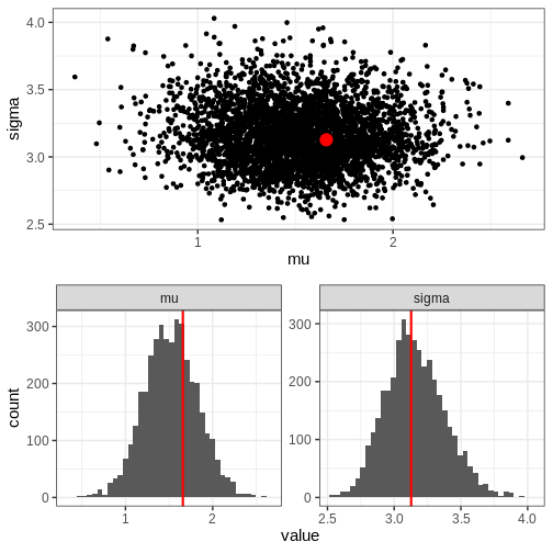
Chain 4: Next, we’ll extract posterior samples and generate a plot for the joint, and marginal posteriors. The true unknown parameter values are included in the plots in red.
R
# Extract parameter samples
par_samples <- rstan::extract(normal_samples, c("mu", "sigma")) %>%
  do.call(cbind, .) %>%
  data.frame


# Full posterior
p_posterior <- ggplot(data = par_samples) +
  geom_point(aes(x = mu, y = sigma)) +
  annotate("point", x = unknown_mu, y = unknown_sigma,
           color = "red", size = 5)

# Marginal posteriors
p_marginals <- ggplot(data = par_samples %>% gather) +
  geom_histogram(aes(x = value), bins = 40) +
  geom_vline(data = data.frame(key = c("mu", "sigma"),
                               value = c(unknown_mu, unknown_sigma)),
             aes(xintercept = value), color = "red", linewidth = 1) +
  facet_wrap(~key, scales = "free")


p <- cowplot::plot_grid(p_posterior, p_marginals,
                        ncol = 1)

print(p)
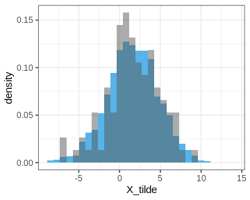
Let’s also plot the posterior predictive distribution samples histogram and compare it to that of the data.
R
PPD <- rstan::extract(normal_samples, c("X_tilde"))[[1]] %>%
  data.frame(X_tilde = . )

p_PPD <- ggplot() +
  geom_histogram(data = PPD,
                 aes(x = X_tilde, y = after_stat(density)),
                 bins = 30, fill = posterior_color) +
  geom_histogram(data = data.frame(X), aes(x = X, y = after_stat(density)),
                 bins = 30, alpha = 0.5)

print(p_PPD)
Example 3: Linear regression
Challenge
Write a Stan program for linear regression with one dependent variable.
Generate data from the linear model and use the Stan program to estimate the intercept \(\alpha\), slope \(\beta\), and noise term \(\sigma\).
STAN
data {
  int<lower=0> N; // Sample size
  vector[N] x; // x-values
  vector[N] y; // y-values
}
parameters {
  real alpha; // intercept
  real beta;  // slope
  real<lower=0> sigma; // noise
}

model {

  // Likelihood
  y ~ normal(alpha + beta * x, sigma);

  // Priors
  alpha ~ normal(0, 1);
  beta ~ normal(0, 1);
  sigma ~ inv_gamma(1, 1);
}
Challenge
Modify the program for linear regression so it facilitates \(M\) dependent variables.
STAN
data {
  int<lower=0> N; // Sample size
  int<lower=0> M; // Number of features
  matrix[N, M] x; // x-values
  vector[N] y; // y-values
}
parameters {
  real alpha; // intercept
  vector[M] beta;  // slopes
  real<lower=0> sigma; // noise
}

model {

  // Likelihood
  y ~ normal(alpha + x * beta, sigma);

  // Priors
  alpha ~ normal(0, 1);
  beta ~ normal(0, 1);
  sigma ~ inv_gamma(1, 1);
}- Stan is a tool for efficient posterior distribution sample generation.
- A Stan program is specified in a separate text file that consists of code blocks, with the data, parameters, and model blocks being the most crucial ones.
Resources
- Official release paper https://www.jstatsoft.org/article/view/v076i01
- User’s guide https://mc-stan.org/docs/2_18/stan-users-guide/
- Function’s reference https://mc-stan.org/docs/functions-reference/
- Reference manual https://mc-stan.org/docs/reference-manual/
- Stan forum https://discourse.mc-stan.org
- Case studies https://mc-stan.org/users/documentation/case-studies
Reading
- BDA3: Ch. 12.6, Appendix C
- Bayes Rules!: Ch. 6.2
Content from Markov chain Monte Carlo
Last updated on 2025-11-10 | Edit this page
Estimated time: 63 minutes
Overview
Questions
- How does Stan generate the posterior samples?
Objectives
Learn
- the basic idea of the Metropolis-Hasting algorithm.
- how to assess Markov chain Monte Carlo convergence.
- how to implement a random walk Metropolis-Hasting algorithm.
The standard solution to fitting probabilistic models is to generate random samples from the posterior distribution. In the previous episode, we learned how to generate posterior samples using Stan without knowing how the samples are generated. In this episode, we’ll study Markov chain Monte Carlo (MCMC) methods, which are the class of algorithms Stan uses under the hood.
Metropolis-Hastings algorithm
MCMC methods draw samples from the posterior distribution by constructing sequences (chains) of values in the parameter space that ultimately converge to the posterior. While there are other variants of MCMC, on this course we will mainly focus on the Metropolis-Hasting (MH) algorithm outlined below. As this algorithm is ran long enough, convergence to posterior (or to other specified target density) is guaranteed. This means that that if the chain is run long enough, the samples will eventually start approximating the posterior distribution.
A chain starts is initialized at value \(\theta^{0}\), which can be manually set or random. The only precondition is that the target distribution has positive mass at the location, \(p(\theta^{0} | X) > 0\). Then, a proposal \(\theta^*\) for the next value is generated from a proposal distribution \(T_i\). An often-used solution is the normal distribution centered at the current value, \(\theta^* \sim N(\theta^{i}, \sigma^2)\). This is where the term “Markov chain” comes from, the value of each element depends only on the previous one.
Next, the proposal \(\theta^*\) is either accepted or rejected. If each proposal was accepted, the sequence would simply be a random walk in the parameter space and would not approximate the posterior to any degree. The rule that determines the acceptance should reflect this; proposals towards higher posterior densities should be favored over proposals toward low density areas. The solution is to compute the ratio
\[r = \frac{p(\theta^* | X) / T_i(\theta^* | \theta^{i})}{p(\theta^i | X) / T_i(\theta^{i} | \theta^{*})},\] and use is as the probability to move to the proposed value. In other words, the next element in the chain is \(\theta^{i+1} = \theta^*\) with probability \(\min(r, 1)\). If the proposal is not accepted the chain stays at the current value, \(\theta^{i+1} = \theta^{i}.\) This approach induces directional randomness in the chain; proposals towards higher density areas are generally accepted but transitions away from it are also possible. In situations where the transition density is symmetric, such as with the normal distribution, \(r\) reduces simply to the ratio of the posterior values, and all proposals toward higher posterior density areas are accepted.
Example: Banana distribution
Let’s implement the MH algorithm and use it to generate posterior samples from the following statistical model:
\[X \sim N(\theta_1 + \theta_2^2, 1) \\ \theta_1, \theta_2 \sim N(0, 1),\]
where \(X\) is univariate data and \(\theta_1, \theta_2\) the parameters.
Helper functions
We begin by writing some helper functions that carry out the incremental steps of the MH algorithm.
First, we need to be able to generate the proposals. Let’s use the
two-dimensional normal with identity covariance scaled by a scalar
jump_scale.
R
set.seed(12)

generate_proposal <- function(pars_now, jump_scale = 0.1) {

  n_pars <- length(pars_now)

  # Random draw from multivariate normal
  theta_star <- mvtnorm::rmvnorm(1,
                                 mean = pars_now,
                                 sigma = jump_scale*diag(n_pars))
  return(theta_star)
}
Running MH also requires computing the (unnormalized) posterior
density at the proposed parameter values. This function returns the log
posterior value at the location pars. The density is
computed on log scale to avoid issues with numerical precision.
R
get_log_target_value <- function(X, pars) {

  # log(likelihood)
  sum(
    dnorm(X,
          mean = pars[1] + pars[2]^2,
          sd = 1,
          log = TRUE)
      ) +

    # log(prior)
    dnorm(pars[1], 0, 1, log = TRUE) +
    dnorm(pars[2], 0, 1, log = TRUE)

}
Then, we’ll write a function that computes the acceptance ratio \(r\). Since the proposal is symmetric, the expression reduces to the ratio of the posterior densities of the proposed and current parameter values. Notice that a ratio on a log scale is equal to the difference of logarithms.
R
# Compute ratio
get_ratio <- function(X, pars_now, pars_proposal) {
  r <- exp(
    get_log_target_value(X, pars_proposal) -
      get_log_target_value(X, pars_now)
    )

  return(r)
}
Finally, we can wrap the helpers in a function that loops over the algorithm steps.
R
# Sampler
MH_sampler <- function(X, # Data
                       inits, # Initial values
                       n_samples = 1000, # Number of iterations
                       jump_scale = 0.1 # Proposal jump variance
                       ) {


  # Matrix for samples
  pars <- matrix(nrow = n_samples, ncol = length(inits))

  # Set initial values
  pars[1, ] <- inits

  # Generate samples
  for(i in 2:n_samples) {

    # Current parameters
    pars_now <- pars[i-1, ]

    # Proposal
    pars_proposal <- generate_proposal(pars_now, jump_scale)

    # Ratio
    r <- get_ratio(X, pars_now, pars_proposal)

    r <- min(1, r)

    # Does the sampler move?
    move <- sample(x = c(TRUE, FALSE),
                   size = 1,
                   prob = c(r, 1-r))
    # OR:
    # move <- runif(n = 1, min = 0, max = 1) <= r

    if(move) {
      pars[i, ] <- pars_proposal
    } else {
      pars[i, ] <- pars_now
    }
  }

  pars <- data.frame(pars)

  return(pars)
}
Run MH
Now we can try out our MH implementation. Let’s use the simulated
data points stored in vector X:
R
X <- c(3.78, 2.76, 2.84, 2.92, 1.3, 3.93, 3.69, 2.28, 2.81, 0.71)
We’ll generate 1000 samples with initial value (0, 5) and jump scale 0.01. The trajectory of samples is plotted over the posterior density computed with the grid approximation.
R
# Draw samples
samples1 <- MH_sampler(X,
                      inits = c(0, 5),
                      n_samples = 1000,
                      jump_scale = 0.01)

colnames(samples1) <- c("theta1", "theta2")

# Add column for sample index
samples1$sample <- 1:nrow(samples1)


# Grid approximation
delta <- 0.05
df_grid <- expand.grid(seq(-4, 4, by = delta),
                       seq(-4, 5, by = delta)) %>%
  set_colnames(c("theta1", "theta2"))


for(i in 1:nrow(df_grid)) {
  df_grid[i, "likelihood"] <- prod(
    dnorm(X,
          df_grid[i, "theta1"] + df_grid[i, "theta2"]^2,
          1)
    )
}

df_grid <- df_grid %>%
  mutate(prior = dnorm(theta1, 0, 1)*dnorm(theta2, 0, 1)) %>%
  mutate(posterior = prior*likelihood) %>%
  mutate(posterior = posterior / (sum(posterior)*delta^2))


# Plot
p_grid <- ggplot() +
  geom_tile(data = df_grid,
             aes(x = theta1, y = theta2, fill = posterior)) +
  scale_fill_gradientn(colours = rainbow(5))


# Plot joint posterior samples
p_MH1 <- p_grid +
  geom_path(data = samples1,
            aes(x = theta1, y = theta2))


print(p_MH1)
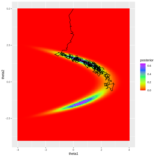
Looking at the figure, a few observations become evident. Firstly, despite the chosen initial value being moderately far from the high-density areas of the posterior, the algorithm quickly converges to the target region. This rapid convergence is due to the fact that proposals toward higher density areas are favored, in fact they are always accepted when using normal density proposals. However, it’s important to note that such swift convergence is not guaranteed in all scenarios. In cases with a high number of model parameters, there’s an increased likelihood of the sampler taking ‘wrong’ directions. The samples before convergence introduce bias to the posterior approximation.
Secondly, the posterior is not fully explored; no samples are generated from the lower mode in the figure. This highlights a crucial point: even if the sampler has converged, it doesn’t guarantee that the drawn samples provide a representative picture of the target.
Challenge
Consider how you could address the two issues raised above:
- Initial unconverged samples introduce a bias.
- The sampler may not have explored the target distribution properly.
Try different proposal distributions variances in the MCMC example
above by changing jump_scale. How does this affect the
inference and convergence? Why?
Assessing convergence
Although convergence of MCMC is theoretically guaranteed, in practice, this is not always the case. Monitoring convergence is crucial whenever MCMC is utilized to ensure the reliability of recovered results.
Depending on the model used, initial values, amount of data, among other factors, can cause convergence issues. Earlier, we mentioned two common complications, and here we will list a few more, along with actions that can alleviate the issues.
Slow convergence can occur when initial values of the chain are far from most of the target mass, resulting in early iterations biasing the approximation. Another cause for slow convergence is that the proposals are not far enough from the current value, and the sampler moves too slowly.
Incomplete exploration: This means that the sampler doesn’t spend enough time in all significant posterior areas.
A large proportion of the proposals is rejected. When the proposal distribution generates proposals too far from the current value, the proposals are rejected and the sampler stands still for many iterations. This leads to inefficiency.
Sample autocorrelation: Consecutive samples are close to each other. Ideally, we’d like to generate independent samples from the target. High sample autocorrelation can be caused by several factors, including the ones mentioned in the previous points.
These issues can be remedied with:
Running multiple long chains with distinct or random initial values.
Discarding the early proportion of the chain as warm-up.
Setting an appropriate proposal distribution.
It also important to be able to monitor whether the sampler has converged. This can be done with statistics, such as effective sample size and \(\hat{R}\). Effective sample size estimates how many independent samples have been generated. Ideally, this number should be close to the total number of iterations the sampler has been ran for. \(\hat{R}\) on the other hand measures chain mixing, that is, how well the chains agree with each other. It is computed by comparing the variance within each chain to the total variance of all samples. Usually, values of \(\hat{R} > 1.1\) are considered as signaling convergence issues. However, the Stan development team recommends using 1.05 as the limit.
Besides statistics, visually evaluating the samples can be useful. Trace plots refer to graphs where the marginal posterior samples are plotted against sample index. Trace plots can be used to investigate convergence and mixing properties, and can reveal, for example, multimodality.
In Stan, many of the above-mentioned points have been automatized. By default, Stan runs 4 chains with 2000 iterations each, and discards the initial 50% as warm-up. Moreover, it computes \(\hat{R}\), effective sample size, and other statistics and throws warnings in case of issues.
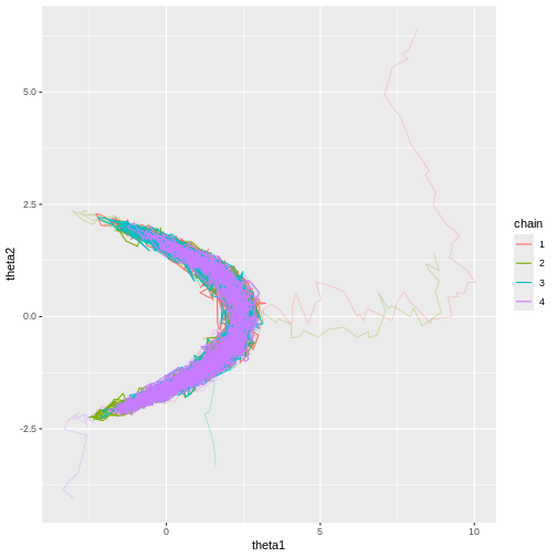
Example continued
In light of the above information, let’s re-fit the model of the previous example. Now, we’ll run 4 chains with random initial values, 10000 samples each, and discard the first 50% of each chain as warm-up. We’ll use 0.1 as the proposal variance.
R
# Number of chains
n_chains <- 4

# Number of samples
n_samples <- 10000

# Initial warmup proportion
warmup <- 0.5

samples2 <- lapply(1:n_chains, function(i) {

  # Use random initial values
  inits <- rnorm(2, 0, 5)

  chain <- MH_sampler(X, inits = inits,
                        n_samples = n_samples,
                        jump_scale = 0.1)

  # Wrangle
  colnames(chain) <- c("theta1", "theta2")
  chain$sample <- 1:nrow(chain)
  chain$chain <- as.factor(i)
  chain[1:round(warmup*n_samples), "warmup"] <- TRUE
  chain[(round(warmup*n_samples)+1):n_samples, "warmup"] <- FALSE

  return(chain)

}) %>%
  do.call(rbind, .)
Now it’s evident that the sample trajectories explore the entire posterior distribution:
R
# Plot
p_joint_2 <- ggplot() +
  # Warm-up samples
  geom_path(data = samples2 %>%
              filter(warmup == TRUE),
            aes(theta1, theta2, color = chain),
            alpha = 0.25) +
  # Post-warm-up samples
  geom_path(data = samples2 %>%
              filter(warmup == FALSE),
            aes(theta1, theta2, color = chain))

print(p_joint_2)
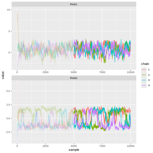
Let’s see what the trace plots look like. Generally, we’d want to see the samples randomly scattered around a mean value. For \(\theta_1\) this is more or less the case, although there some autocorrelation is apparent. With \(\theta_2\) we can see that the chains have mixed as they explore the same parameter ranges. However, the bimodality of the posterior is quite apparent. The \(\hat{R}\) statistics are 1.0082279 and 1.1065365 for \(\theta_1\) and \(\theta_2\), respectively.
R
# Trace plots
p_trace_2 <- ggplot() +
  geom_line(data = samples2 %>%
              filter(warmup == TRUE) %>%
              gather(key = "parameter",
                     value = "value",
                     -c("sample", "chain", "warmup")),
            aes(x = sample, y = value, color = chain),
            alpha = 0.25) +
  geom_line(data = samples2 %>%
              filter(warmup == FALSE) %>%
              gather(key = "parameter",
                     value = "value",
                     -c("sample", "chain", "warmup")),
            aes(x = sample, y = value, color = chain)) +
  facet_wrap(~parameter,
             ncol = 1,
             scales = "free")


print(p_trace_2)
Hamiltonian Monte Carlo
Stan uses a variant of the Metropolis-Hastings algorithm called Hamiltonian Monte Carlo (HMC; or actually a variant HMC). The defining feature is the elaborate scheme it uses to generate proposals. Briefly, the idea is to simulate the dynamics of a particle moving in a potential landscape defined by the posterior. At each iteration, the particle is given a random momentum vector and then its dynamics are simulated forward for some time. The end of the trajectory is then taken as the proposal value.
Compared to the random walk Metropolis-Hastings we implemented in this episode, HMC is very efficient. The main advantages of HMC is its ability to explore high-dimensional spaces more effectively, making it especially useful in complex models with many parameters.
A type of convergence criterion exclusive to HMC is the divergent transition. In a region of the parameter space where the posterior has high curvature, the simulated particle dynamics can produce spurious transitions which do not represent the posterior accurately. Such transitions are called divergent and signal that the particular area of parameter space is not explored accurately. Stan provides information about divergent transitions automatically.
- Markov chain Monte Carlo methods can be used to generate samples from a posterior distribution.
- Values of the chain are generated from a proposal distribution.
- Proposals towards higher areas of the target distribution are accepted with higher probability.
- MCMC convergence should always be monitored.
Reading
See interactive visualization of different MCMC algorithms: https://chi-feng.github.io/mcmc-demo/app.html
Bayesian Data Analysis (3rd ed.): Ch. 11-12
Statistical Rethinking (2nd ed.): Ch. 9
Bayes Rules!: Ch. 6-7
Content from Hierarchical models
Last updated on 2025-11-10 | Edit this page
Estimated time: 14 minutes
Overview
Questions
- How does Bayesian modeling accommodate group structure?
Objectives
- Learn to construct and fit hierarchical models.
Hierarchical (or multi-level) models are a class of models suited for situations where the study population comprises distinct but interconnected groups. For example, analyzing student performance across different schools, income disparities among various regions, or studying animal behavior within different populations are scenarios where such models would be appropriate.
Incorporating group-wise parameters allows us to model each group separately, and a model becomes hierarchical when we treat the parameters of the prior distribution as unknown. These parameters, known as hyperparameters, are assigned their own prior distribution, referred to as a hyperprior, and are learned during the model fitting process. Similarly as priors, the hyperpriors should be set so they reflect ranges of possible hyperparameter values. Conceptually, these hyperparameters and hyperpriors operate at a higher level of hierarchy, hence the name.
For example, let’s consider the beta-binomial model discussed in Episode 1. We used it to estimate the prevalence of left-handedness based on a sample of 50 students. If we were to include additional information, such as the students’ majors, we could extend the model as follows:
\[X_g \sim \text{Bin}(N_g, \theta_g) \\ \theta_g \sim \text{Beta}(\alpha, \beta) \\ \alpha, \beta \sim \Gamma(2, 0.1).\]
Here, the subscript \(g\) indexes the groups based on majors. The group-specific prevalences for left-handedness \(\theta_g\) are assigned a beta prior with hyperparameters \(\alpha\) and \(\beta\) which are treated as random variables. The final line indicates the hyperprior \(\Gamma(2, 0.1)\) governing the prior beliefs about the hyperparameters.
In this hierarchical beta-binomial model, students are considered exchangeable within their majors but no longer across the entire population. However, an underlying assumption of similarity exists between the groups since they share a common prior, that is learned. This way the groups are not entirely independent but are not treated as equal either.
One of the key advantages of Bayesian hierarchical models is their capacity to leverage information across groups. By pooling information from various groups, these models can yield more robust estimates, particularly when data availability is limited.
Another distinction from non-hierarchical models is that the prior, or the population distribution, of the parameters is learned in the process. This population distribution can provide information into parameter variability on a broader scale, even for groups where data is scarce or completely missing. For instance, if we had data on the handedness of students majoring in natural sciences, the population distribution can give insights into students in humanities and social sciences as well.
In the following example, we will perform a hierarchical analysis of human heights across different countries.
Example: human height
Let’s examine the heights of adults in various countries. In [1], averages and standard errors of adult heights in centimeters across different countries and age groups were provided. We’ll utilize this dataset to generate a sample of hypothetical individual heights and then assess our ability to reproduce these measured height statistics.
This approach is commonly employed when building and testing models: we generate simulated data with known parameters and then compare the inferred results to these known parameters. In our case, the true parameters are derived from real-world data.
We’ll employ a normal model with unknown mean \(\mu\) and standard deviation \(\sigma\) as our generative model, and treat these parameters hierarchically.
First, let’s load the data and examine its structure.
R
set.seed(4985)

height <- read.csv("data/height_data.csv")
str(height)
OUTPUT
'data.frame':	210000 obs. of  8 variables:
 $ Country                                   : chr  "Afghanistan" "Afghanistan" "Afghanistan" "Afghanistan" ...
 $ Sex                                       : chr  "Boys" "Boys" "Boys" "Boys" ...
 $ Year                                      : int  1985 1985 1985 1985 1985 1985 1985 1985 1985 1985 ...
 $ Age.group                                 : int  5 6 7 8 9 10 11 12 13 14 ...
 $ Mean.height                               : num  103 109 115 120 125 ...
 $ Mean.height.lower.95..uncertainty.interval: num  92.9 99.9 106.3 112.2 117.9 ...
 $ Mean.height.upper.95..uncertainty.interval: num  114 118 123 128 132 ...
 $ Mean.height.standard.error                : num  5.3 4.72 4.27 3.92 3.66 ...
Let’s subset this data to simplify the analysis and focus on the height of adult women measured in 2019.
R
height_women <- height %>%
  filter(
    Age.group == 19,
    Sex == "Girls",
    Year == 2019
    ) %>%
  # Select variables of interest
  select(Country, Sex, Mean.height, Mean.height.standard.error)
Let’s select 10 countries randomly
R
set.seed(5431)
# Select countries
N_countries <- 10
Countries <- sample(unique(height_women$Country),
                    size = N_countries,
                    replace = FALSE) %>% sort

height_women10 <- height_women %>% filter(Country %in% Countries)

height_women10
OUTPUT
         Country   Sex Mean.height Mean.height.standard.error
1     Bangladesh Girls    152.3776                  0.4966124
2         Belize Girls    158.1201                  1.4026324
3       Cameroon Girls    160.4112                  0.6146315
4           Chad Girls    162.1242                  0.8894219
5  Cote d'Ivoire Girls    158.6524                  0.9254438
6          Ghana Girls    158.8551                  0.8002225
7          Kenya Girls    159.4338                  0.6680202
8     Luxembourg Girls    165.0690                  1.3778094
9         Taiwan Girls    160.6953                  0.7307839
10     Venezuela Girls    160.0370                  1.0813162
Simulate data
Now, we can treat the values in the table above as ground truth and simulate some data based on them. Let’s generate \(N=10\) samples for each country from the normal model with \(\mu = \text{Mean.height}\) and \(\sigma = \text{Mean.height.standard.error}\).
R
# Sample size per group
N <- 10

# For each country, generate heights
height_sim <- lapply(1:N_countries, function(i) {

  my_df <- height_women10[i, ]

  data.frame(Country = my_df$Country,
             # Random values from normal
             Height = rnorm(N,
                            mean = my_df$Mean.height,
                            sd = my_df$Mean.height.standard.error))

}) %>%
  do.call(rbind, .)
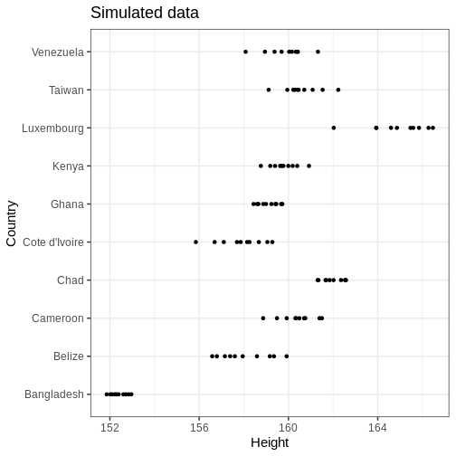
Let’s plot the data
R
# Plot
height_sim %>%
    ggplot() +
    geom_point(aes(x = Height, y = Country)) +
    labs(title = "Simulated data")
Modeling
Let’s build a normal model that uses partial pooling for the country means and standard deviations. The model can be stated as follows:
\[\begin{align} X_{gi} &\sim \text{N}(\mu_g, \sigma_g) \\ \mu_g &\sim \text{N}(\mu_\mu, \sigma_\mu) \\ \sigma_g &\sim \Gamma(\alpha_\sigma, \beta_\sigma) \\ \mu_\mu &\sim \text{N}(0, 100)\\ \sigma_\mu &\sim \Gamma(2, 0.1) \\ \alpha_\sigma, \beta_\sigma &\sim \Gamma(2, 0.01). \end{align}\]
Above, \(X_{gi}\) denotes the height for individual \(i\) in country \(g\). The country specific parameters \(\mu_g\) and \(\sigma_g\) are given normal and gamma priors, respectively, with unknown hyperparameters that, in turn, are given hyperpriors on the last two lines. The hyperpriors are quite uninformative as they allow large hyperparameter ranges.
Below is the Stan program for this model. The data points are input
as a concatenated vector X. The country-specific start and
end indices are computed in the transformed data block. This approach
accommodates uneven sample sizes between groups, although in our data
these are equal.
The parameters block contains the declarations of mean and standard deviation vectors, along with the hyperparameters. The hyperparameter subscripts denote the parameter they are assigned to so, for instance, \(\sigma_{\mu}\) is the standard deviation of the mean parameter \(\mu\). The generated quantities block generates samples from the population distributions of \(\mu\) and \(\sigma\) and a country-agnostic posterior predictive distribution \(\tilde{X}\).
STAN
data {
  int<lower=0> G; // number of groups
  int<lower=0> N[G]; // sample size within each group
  vector[sum(N)] X; // concatenated observations
}

transformed data {
  // get first and last index for each group in X
  int start_i[G];
  int end_i[G];

  for(g in 1:G) {

    if(g == 1) {
      start_i[1] = 1;
    } else {
      start_i[g] = start_i[g-1] + N[g-1];
    }

    end_i[g] = start_i[g] + N[g]-1;
  }
}

parameters {

  // parameters
  vector[G] mu;
  vector<lower=0>[G] sigma;

  // hyperparameters
  real mu_mu;
  real<lower=0> sigma_mu;
  real<lower=0> alpha_sigma;
  real<lower=0> beta_sigma;
}

model {

  // Likelihood for each group
  for(i in 1:G) {
    X[start_i[i]:end_i[i]] ~ normal(mu[i], sigma[i]);
  }

  // Priors
  mu ~ normal(mu_mu, sigma_mu);
  sigma ~ gamma(alpha_sigma, beta_sigma);

  // Hyperpriors
  mu_mu ~ normal(0, 100);
  sigma_mu ~ gamma(2, 0.1);
  alpha_sigma ~ gamma(2, 0.01);
  beta_sigma ~ gamma(2, 0.01);
}

generated quantities {

  real mu_tilde;
  real<lower=0> sigma_tilde;
  real X_tilde;

  // Population distributions
  mu_tilde = normal_rng(mu_mu, sigma_mu);
  sigma_tilde = gamma_rng(alpha_sigma, beta_sigma);

  // Posterior predictive distribution
  X_tilde = normal_rng(mu_tilde, sigma_tilde);

}
Now we can call Stan and fit the model. Hierarchical models can
encounter convergence issues and for this reason, we’ll use 10000
iterations and set adapt_delta = 0.99. This controls the
acceptance probability in Stan’s adaptation period and will result in a
smaller step size in the Markov chain. Moreover, we’ll speed up the
inference by running 2 chains in parallel by setting
cores = 2.
R
stan_data <- list(G = length(unique(height_sim$Country)),
                  N = rep(N, length(Countries)),
                  X = height_sim$Height)

normal_hier_fit <- rstan::sampling(normal_hier_model,
                                   stan_data,
                                   iter = 10000,
                                   chains = 2,
                                   # Use to avoid divergent transitions:
                                   control = list(adapt_delta = 0.99),
                                   cores = 2)
For comparison, we will also run an unpooled analysis of heights, which makes use of the following Stan file:
R
unpooled_summaries <- list()

for(i in 1:N_countries) {

  my_country <- unique(height_sim$Country)[i]

  my_df <- height_sim %>%
    filter(Country == my_country)

  my_stan_data <- list(N =  my_df %>% nrow,
                       X = my_df$Height)

  my_fit <- rstan::sampling(normal_pooled_model,
                              my_stan_data,
                              iter = 10000,
                              chains = 2,
                                    # Use to get rid of divergent transitions:
                                    control = list(adapt_delta = 0.99),
                              cores = 2,
                            refresh = 0
                            )


  unpooled_summaries[[i]] <- rstan::summary(my_fit, c("mu", "sigma"))$summary %>%
  data.frame() %>%
  rownames_to_column(var = "par") %>%
  mutate(country = my_country)

}


unpooled_summaries <- do.call(rbind, unpooled_summaries)
Country-specific estimates
Let’s first compare the marginal posteriors for the country-specific estimates from the hierarchical model (blue) and an unpooled model (brown) that treats the parameters separately.
R
par_summary <- rstan::summary(normal_hier_fit, c("mu", "sigma"))$summary %>%
  data.frame() %>%
  rownames_to_column(var = "par") %>%
  separate(par, into = c("par", "country"), sep = "\\[") %>%
  mutate(country = gsub("\\]", "", country)) %>%
  mutate(country = Countries[as.integer(country)])

ggplot() +
geom_errorbar(data = par_summary, aes(x = country, ymin = X2.5., ymax = X97.5.),
              color = posterior_color) +
geom_point(data = height_women10 %>%
             rename_with(~ c('mu', 'sigma'), 3:4) %>%
             gather(key = "par",
                    value = "value",
                    -c(Country, Sex)),
           aes(x = Country, y = value)) +
geom_errorbar(data = unpooled_summaries,
              aes(x = country, ymin = X2.5., ymax = X97.5.),
              color = "brown") +
facet_wrap(~ par, scales = "free", ncol = 1) +
coord_flip()
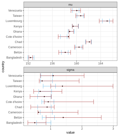
Above, the black points represent the true values, and the intervals are the 95% CIs for a hierarchical and non-hierarchical models, respectively. As apparent, the CIs from the hierarchical model are more concentrated and better capture the true values.
Challenge
Experiment with the data and fit. Explore the effect of sample size, unequal sample sizes between countries, and the amount of countries, for example.
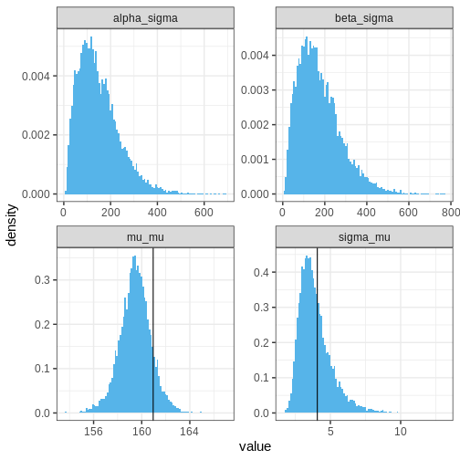
Hyperparameters
Let’s then plot the population distribution’s parameters, that is, the hyperparameters. The sample-based values are included in the plots of \(\mu_\mu\) and \(\sigma_\mu\) (why not for the other two hyperparameters?). It seems that the model has slightly underestimated the overall average and variance of the mean parameter \(\mu\), which is not suprising given the low number of data points.
R
## Population distributions:
population_samples_l <- rstan::extract(normal_hier_fit,
                                       c("mu_mu", "sigma_mu", "alpha_sigma", "beta_sigma")) %>%
  do.call(cbind, .) %>%
  set_colnames(c("mu_mu", "sigma_mu", "alpha_sigma", "beta_sigma")) %>%
  data.frame() %>%
  mutate(sample = 1:nrow(.)) %>%
  gather(key = "hyperpar", value = "value", -sample)


ggplot() +
  geom_histogram(data = population_samples_l,
                 aes(x = value, y = after_stat(density)),
                 fill = posterior_color,
                 bins = 100) +
  geom_vline(data = height_women %>%
               rename_with(~ c('mu', 'sigma'), 3:4) %>%
               filter(Sex == "Girls") %>%
               summarise(mu_mu = mean(mu), sigma_mu = sd(mu)) %>%
               gather(key = "hyperpar", value = "value"),
             aes(xintercept = value)
             )+
  facet_wrap(~hyperpar, scales = "free")
Population distributions
Let’s then plot the population distributions and compare to the true sample means and standard errors.
R
population_l <- rstan::extract(normal_hier_fit, c("mu_tilde", "sigma_tilde")) %>%
  do.call(cbind, .) %>%
  data.frame() %>%
  set_colnames( c("mu", "sigma")) %>%
  mutate(sample = 1:nrow(.)) %>%
  gather(key = "par", value = "value", -sample)


ggplot() +
  geom_histogram(data = population_l,
                 aes(x = value, y = after_stat(density)),
                 bins = 100, fill = posterior_color) +
    geom_histogram(data = height_women %>%
                     rename_with(~ c('mu', 'sigma'), 3:4) %>%
                     gather(key = "par", value = "value", -c(Country, Sex)) %>%
                     filter(Sex == "Girls"),
                   aes(x = value, y = after_stat(density)),
                   alpha = 0.75, bins = 30) +
  facet_wrap(~par, scales = "free") +
  labs(title = "Blue = posterior; black = sample")
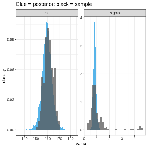 We can see that the population distribution is able to capture the
measured average heights and standard deviations relatively well,
although the within-country variation is estimated to be too
concentrated. However, remember that these estimates are based on a
limited sample: 10 out of 200 countries with 10 individuals in each
group.
We can see that the population distribution is able to capture the
measured average heights and standard deviations relatively well,
although the within-country variation is estimated to be too
concentrated. However, remember that these estimates are based on a
limited sample: 10 out of 200 countries with 10 individuals in each
group.
Posterior predictive distribution
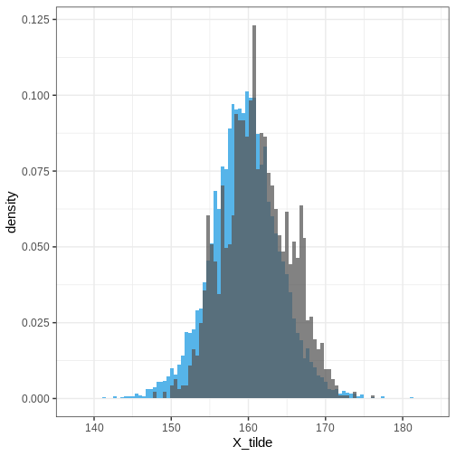
Finally, let’s plot the posterior predictive distribution for the whole population and overlay it with the simulated data based on all countries.
R
# For each country, generate some random girl's heights
height_all <- lapply(1:nrow(height_women), function(i) {

  my_df <- height_women[i, ] %>%
    rename_with(~ c('mu', 'sigma'), 3:4)

  data.frame(Country = my_df$Country,
             Sex = my_df$Sex,
             # Random normal values based on sample mu and sd
             Height = rnorm(N, my_df$mu, my_df$sigma))

}) %>%
  do.call(rbind, .)
R
# Extract the posterior predictive distribution
PPD <- rstan::extract(normal_hier_fit, c("X_tilde")) %>%
  data.frame() %>%
  set_colnames( c("X_tilde")) %>%
  mutate(sample = 1:nrow(.))


ggplot() +
  geom_histogram(data = PPD,
                 aes(x = X_tilde, y = after_stat(density)),
                 bins = 100,
                 fill = posterior_color) +
  geom_histogram(data = height_all,
                 aes(x = Height, y = after_stat(density)),
                 alpha = 0.75,
                 bins = 100)
Extensions
Here, we analyzed the height for women in a randomly chosen countries using a hierarchical model. The model could be extended further, for instance, by adding hierarchy between sexes, continents, developed/developing countries etc.
- Hierarchical models are appropriate for scenarios where the study population naturally divides into subgroups.
- Hierarchical models borrow statistical strength across the population groups.
- Population distributions hold information about the variation of the model parameters over the whole population.
Reading
- Bayesian Data Analysis (3rd ed.): Ch. 5
- Statistical Rethinking (2nd ed.): Ch. 13
- Bayes Rules!: Ch. 15-19
References
[1] Height: Height and body-mass index trajectories of school-aged children and adolescents from 1985 to 2019 in 200 countries and territories: a pooled analysis of 2181 population-based studies with 65 million participants. Lancet 2020, 396:1511-1524
Content from Model comparison
Last updated on 2025-11-10 | Edit this page
Estimated time: 62 minutes
Overview
Questions
- How can competing models be compared?
Objectives
Get a basic understanding of comparing models with
posterior predictive check
information criteria
Bayesian cross-validation
There is often uncertainty about which model would be the most appropriate choice a data being analysed. The aim of this episode is to introduce some tools that can be used to compare models systematically. We will explore three different approaches.
The first one is the posterior predictive check, which involves comparing a fitted model’s predictions with the observed data. The second approach is to use information criteria, which measure the balance between model complexity and goodness-of-fit. The episode concludes with Bayesian cross-validation.
Data
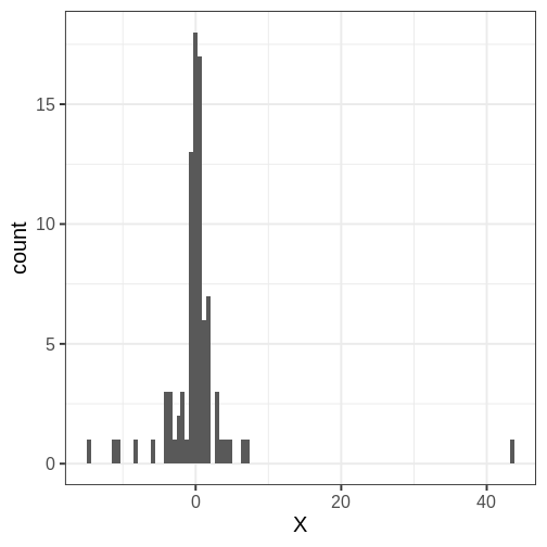
Throughout the chapter, we will use the same simulated data set in the examples, a set of \(N=88\) univariate numerical data points. The data is included in the course’s data folder at
Looking at the data histogram, it’s evident that the data is approximately symmetrically distributed around 0. However, there is some dispersion in the data, and an extreme positive value, suggesting that the tails might be longer than those of a normal distribution. The Cauchy distribution is a potential alternative and below we will compare the suitability of these two distributions on this data.
Posterior predictive check
The idea of posterior predictive checking is to use the posterior predictive distribution to simulate a replicate data set and compare it to the observed data. The reasoning behind this approach is that if the model is a good fit, then replicate data should look similar the observed one. Qualitative discrepancies between the simulated and observed data can imply that the model does not match the properties of the data or the domain.
The comparison can be done in different ways. Visual comparison is an option but a more rigorous approach is to compute the posterior predictive p-value (\(p_B\)), which measures how well the model can reproduce the observed data. Computing the \(p_B\) requires specifying a statistic whose value is compared between the posterior predictions and the observations.
The steps of a posterior predictive check can be formulated in the following points:
- Generate replicate data: Use the posterior predictive distribution to simulate replicate datasets \(X^{rep}\) with characteristics matching the observed data. In our example, this amounts to generating data with \(N=88\) for each posterior sample.
- Choose test quantity \(T(X)\): Choose an aspect of the data that you wish to check. We’ll use the maximum value as the test quantity and compute it for the observed data and each replicate. It’s important to note that not every imaginable data quantity will make a good \(T(X)\), see chapter 6.3 in BDA3 for details.
- Compute \(p_B\): The posterior predictive p-value is defined as the probability \(Pr(T(X^{rep}) \geq T(X) | X)\), that is, the probability that the predictions produce test quantity values at least as extreme as those found in the data. Using samples, it is computed as the proportion of replicate data sets with \(T\) not smaller than that of \(T(X)\). The closer the \(p_B\)-value is to 1 (or 0), the larger the evidence that the model cannot properly emulate the data.
Next we will perform these steps for the normal and Cauchy models.
Normal model
Below is a Stan program for the normal model that produces the
replicate data in the generated quantities block. The values of
X_rep are generated in a loop using the random number
generator normal_rng. Notice that a single posterior sample
\((\mu_s, \sigma_s)\) is used for each
evaluation of the generated quantities block, resulting in a
distribution of \(X^{rep}\)
STAN
data {
  int<lower=0> N;
  vector[N] X;
}
parameters {
  real<lower=0> sigma;
  real mu;
}
model {
  X ~ normal(mu, sigma);

  mu ~ normal(0, 1);
  sigma ~ gamma(2, 1);
}

generated quantities {
  vector[N] X_rep;

  for(i in 1:N) {
    X_rep[i] = normal_rng(mu, sigma);
  }
}
Let’s fit model and extract the replicates.
R
# Fit
normal_fit <- sampling(normal_model,
                       list(N = N, X = df5$X),
                       refresh = 0)

# Extract
X_rep <- rstan::extract(normal_fit, "X_rep")[[1]] %>%
  data.frame() %>%
  mutate(sample = 1:nrow(.))
Below is a comparison of 9 realizations of \(X^{rep}\) (blue) against the data (grey; the panel titles correspond to MCMC sample numbers). It is evident that the tail properties are different between \(X^{rep}\) and \(X\), and this discrepancy indicates an issue with the model choice.
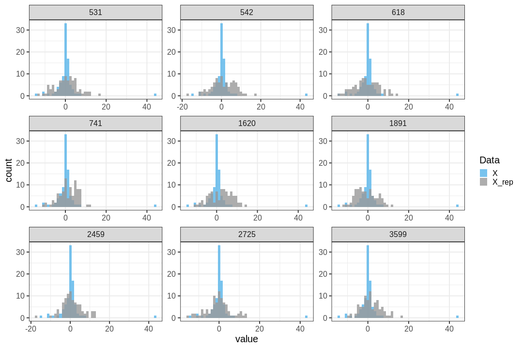
Let’s quantify this discrepancy by computing the \(p_B\) using the maximum of the data as a test statistic. The maximum of the original data is max(\(X\)) = 43.481. The posterior predictive \(p\)-value is \(p_B =\) 0.
This means that the chosen statistic \(T\) is at least as large as in the data in 100% of the replications, indicating strong evidence that the normal model is a poor choice for the data.
The following histogram displays \(T(X) = \max(X)\) (vertical line) against the distribution of \(T(X^{rep})\).
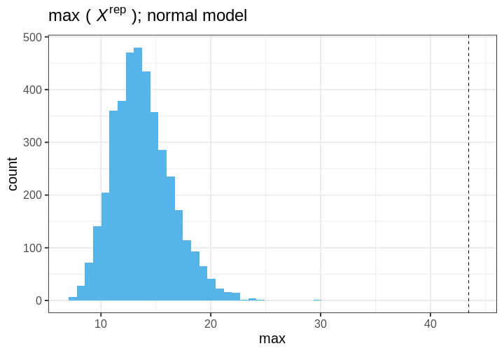
Cauchy model
Let’s do an identical analysis using the Cauchy model.
The results are generated with code essentially copy-pasted from above, with a minor distinction in the Stan program.
STAN
data {
  int<lower=0> N;
  vector[N] X;
}
parameters {
  // Scale
  real<lower=0> sigma;
  // location
  real mu;
}
model {
  // location = mu and scale = sigma
  X ~ cauchy(mu, sigma);

  mu ~ normal(0, 1);
  sigma ~ gamma(2, 1);
}
generated quantities {
  vector[N] X_rep;
  for(i in 1:N) {
    X_rep[i] = cauchy_rng(mu, sigma);
  }
}
A comparison of data \(X\) and \(X^{rep}\) from the Cauchy model shows good agreement between the posterior predictions and the data. The distributions appear to closely match around 0, and the replicates contain some extreme values similarly to the data.
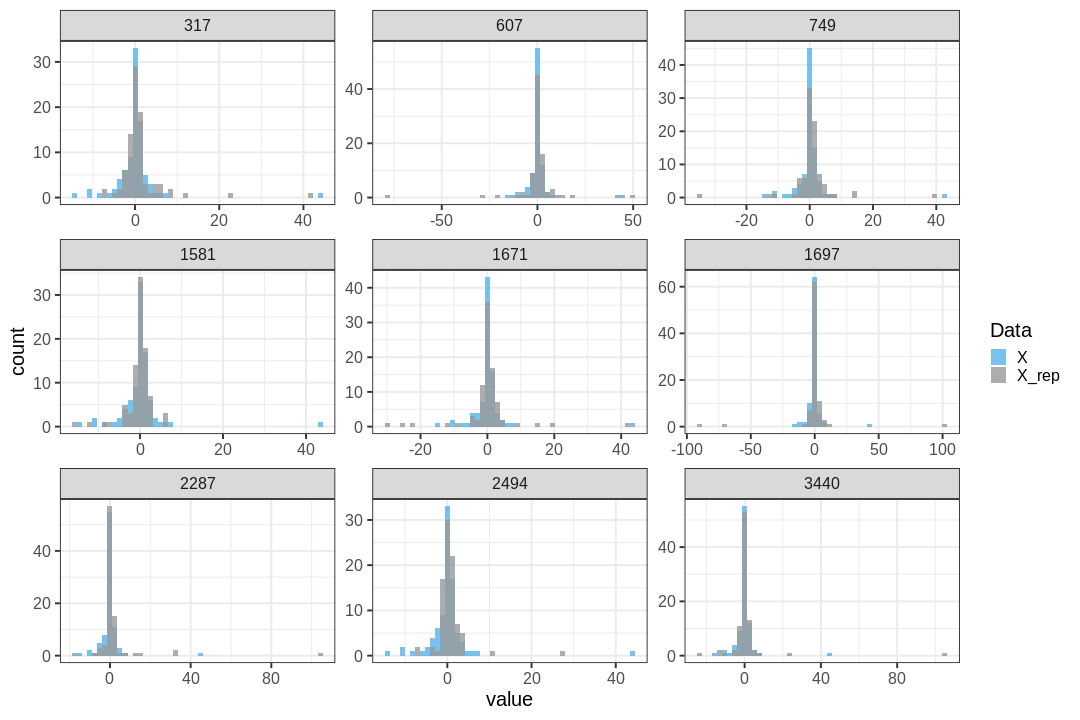
The maximum value observed in the data is similar to those from replicate sets. Additionally, \(p_B=\) 0, indicating no issues with the suitability of the model for the data. distribution.
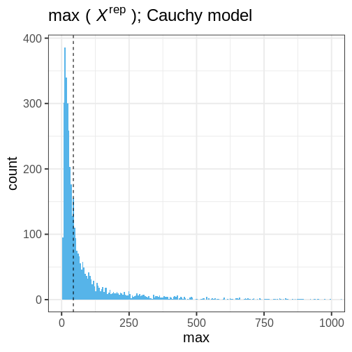
Information criteria
Information criteria are statistics used for model comparison within both Bayesian and classical frequentist frameworks. These criteria provide a means to compare the relative suitability of a model to data by estimating out-of-sample predictive accuracy while simultaneously taking model complexity into account.
The Widely Applicable Information Criterion (WAIC) is an information criteria developed within the Bayesian framework. WAIC is computed using the log pointwise predictive density (lppd) of the data. Since the predictions are based on the model fit with the the data lppd is an overly confident estimate of the predictive capability. To take this into account, a penalization term \(p_{WAIC}\) is included:
\[WAIC = -2(\text{lppd} - p_{WAIC}).\] The log pointwise predictive density is computed as ${i=1}^N({s=1}^Sp(X_i | ^s)), $, where \(X_i, \,i=1,\ldots,N\) are data points and \(S\) the number of posterior samples. The penalization term \(p_{WAIC} = \sum_{i=1}^N \text{Var}(\log p(y_i | \theta^s))\) measures the effective number of parameters (although this may not be apparent from the formula). Because the definition contains a negative of the difference \(\text{lppd} - p_{WAIC}\), lower WAIC values imply a better fit.
Let’s use the WAIC to compare the normal and Cauchy models. First we’ll need to fit both models on the data using the Stan programs utilized above.
R
stan_data <- list(N = N, X = df5$X)

# Fit
normal_fit <- sampling(normal_model, stan_data,
                       refresh = 0)
cauchy_fit <- sampling(cauchy_model, stan_data,
                       refresh = 0)

# Extract samples
normal_samples <- rstan::extract(normal_fit, c("mu", "sigma")) %>%
  data.frame
cauchy_samples <- rstan::extract(cauchy_fit, c("mu", "sigma")) %>%
  data.frame
Then we will write a function for computing WAIC, but first a helper function to compute posterior predictive density for a single point.
R
get_ppd_point <- function(x, samples, model) {

  # Loop over posterior samples
  pp_dens <- lapply(1:nrow(samples), function(S) {

    my_mu <- samples[S, "mu"]
    my_sigma <- samples[S, "sigma"]

    if(model == "normal") {
      # Normal(x | mu, sigma^2)
      dnorm(x = x,
            mean = my_mu,
            sd = my_sigma)
    } else if (model == "cauchy") {
      # Cauchy(x | location = mu, scale = sigma^2)
      dcauchy(x = x,
              location = my_mu,
              scale = )
    }

  }) %>%
    unlist()

  return(pp_dens)
}

WAIC <- function(samples, data, model){

  # Loop over data points
  pp_dens <- lapply(1:length(data), function(i) {
    get_ppd_point(data[i], samples, model)
  }) %>%
    do.call(rbind, .)

  lppd <- apply(X = pp_dens,
                MARGIN = 1,
                FUN = function(x) log(mean(x))) %>%
    sum

  bias <- apply(X = pp_dens,
                MARGIN = 1,
                FUN = function(x) var(log(x))) %>%
    sum

  # WAIC
  waic = -2*(lppd - bias)

  return(waic)
}
Applying this function to the posterior samples, we’ll obtain a lower value for the Cauchy model, implying a better fit to the data. This is in line with the posterior predictive check performed above.
R
WAIC(normal_samples, df5$X, model = "normal")
OUTPUT
[1] 582.6821R
WAIC(cauchy_samples, df5$X, model = "cauchy")
OUTPUT
[1] 412.4815Bayesian cross-validation
The final approach we take to model comparison in cross-validation.
Cross-validation is a technique that estimates how well a model predicts previously unseen data by using fits of the model to a subset of the data to predict the rest of the data.
Performing cross-validation entails defining data partitioning for model training and testing. The larger the proportion of the data used for training, the better the accuracy. However, increasing the size of training data leads to having to fit the model more times. In the extreme case, when each data point is left out individually, the model is fit \(N\) times. This is called leave-one-out cross-validation.
To evaluate the predictive accuracy we will use log predictive
density and take the sum over the different fits as the measure
accuracy. This is then compared to the predictive densities of the data
points based on the fit with all the data. This difference represents
the effective number of parameters \(p_{\text{loo-cv}}\) that can be used for
comparing models.
\[p_{\text{loo-cv}} = \text{lppd} -
\text{lppd}_\text{loo-cv}.\] Above, \(\text{lppd}_\text{loo-cv}\) is the sum of
the log predictive densities of data points evaluated based on
Let’s implement this in R.
R
# Loop over data partitions
normal_loo_lpds <- lapply(1:N, function(i) {

  # Subset data
  my_X <- X[-i]
  my_x <- X[i]

  # Fit model
  my_normal_fit <- sampling(normal_model,
                            list(N = length(my_X),
                                 X = my_X),
                            refresh = 0
                            )

  # Samples
  my_samples <- rstan::extract(my_normal_fit, c("mu", "sigma")) %>%
    do.call(cbind, .) %>%
    set_colnames(c("mu", "sigma"))

  # lppd
  my_lppd <- get_ppd_point(my_x, my_samples, "normal") %>%
    mean %>% log

  data.frame(i, lppd = my_lppd, model = "normal_loo")

}) %>%
  do.call(rbind, .)

# Same for Cauchy:
cauchy_loo_lpds <- lapply(1:N, function(i) {

 # Subset data
  my_X <- X[-i]
  my_x <- X[i]

  # Fit model
  my_cauchy_fit <- sampling(cauchy_model,
                            list(N = length(my_X),
                                 X = my_X),
                            refresh = 0
                            )

  # Samples
  my_samples <- rstan::extract(my_cauchy_fit, c("mu", "sigma")) %>%
    do.call(cbind, .) %>%
    set_colnames(c("mu", "sigma"))

  # lppd
  my_lppd <- get_ppd_point(my_x, my_samples, "cauchy") %>%
    mean %>% log

  data.frame(i, lppd = my_lppd, model = "cauchy_loo")

}) %>%
  do.call(rbind, .)


# Predictive density for data points using full data in training
normal_full_lpd <- lapply(1, function(dummy) {

  # Fit model
  my_normal_fit <- sampling(normal_model,
                            list(N = length(X),
                                 X = X),
                            refresh = 0)

  # Get data
  my_samples <- rstan::extract(my_normal_fit, c("mu", "sigma")) %>%
    do.call(cbind, .) %>%
    set_colnames(c("mu", "sigma"))

  # Compute lppd
  lppds <- lapply(1:N, function(i) {

    my_lppd <- get_ppd_point(X[i], my_samples, "normal") %>%
      mean %>% log

    data.frame(i, lppd = my_lppd, model = "normal")
  }) %>% do.call(rbind, .)

  return(lppds)
}) %>%
  do.call(rbind, .)

cauchy_full_lpd <- lapply(1, function(dummy) {

  # Fit model
  my_cauchy_fit <- sampling(cauchy_model,
                            list(N = length(X),
                                 X = X),
                            refresh = 0)

  # Get data
  my_samples <- rstan::extract(my_cauchy_fit, c("mu", "sigma")) %>%
    do.call(cbind, .) %>%
    set_colnames(c("mu", "sigma"))

  # Compute lppd
  lppds <- lapply(1:N, function(i) {

    my_lppd <- get_ppd_point(X[i], my_samples, "cauchy") %>%
      mean %>% log

    data.frame(i, lppd = my_lppd, model = "cauchy")
  }) %>% do.call(rbind, .)

  return(lppds)
}) %>%
  do.call(rbind, .)
Let’s combine the computed log densities, and compute model-wise sums
R
# Combine
lppds <- rbind(normal_loo_lpds,
              normal_full_lpd,
              cauchy_loo_lpds,
              cauchy_full_lpd)

lppd_summary <- lppds %>%
  group_by(model) %>%
  summarize(lppd = sum(lppd))
Finally, we can compute the estimated of the effective number of parameters. As with WAIC, smaller values imply better suitability. In line with the posterior predictive check and WAIC, we see that, again, the Cauchy distribution gives a better description of the data that the normal model.
R
# Effective number of parameters
p_loo_cv_normal <- lppd_summary[lppd_summary$model == "normal", "lppd"] - lppd_summary[lppd_summary$model == "normal_loo", "lppd"]
p_loo_cv_cauchy <- lppd_summary[lppd_summary$model == "cauchy", "lppd"] - lppd_summary[lppd_summary$model == "cauchy_loo", "lppd"]


paste0("Effective number of parameters, normal = ", p_loo_cv_normal)
OUTPUT
[1] "Effective number of parameters, normal = 33.1191161913168"R
paste0("Effective number of parameters, cauchy = ", p_loo_cv_cauchy)
OUTPUT
[1] "Effective number of parameters, cauchy = 0.79387837262459"There are packages that enable computing WAIC and approximate leave-one-out score automatically so, in practice, there is seldom need to implement these yourself. In episode 7 you will learn about these options tools.
- Bayesian model comparison can be performed (for example) with posterior predictive checks, information criteria, and cross-validation.
Reading
Statistical Rethinking: Ch. 7
BDA3: p.143: 6.3 Posterior predictive checking
PSIS-loo
Content from Gaussian processes
Last updated on 2025-11-10 | Edit this page
Estimated time: 63 minutes
Overview
Questions
- How to do probabilistic non-parameteric regression?
Objectives
- Learn to perform Gaussian process regression with Stan
Gaussian processes (GPs) are a class of stochastic (random) processes that are widely used for non-parametric regression, that is, when the relationship between the predictors and the dependent variable has no parametric form. Formally, a Gaussian process \(GP(\mu, K)\) is defined as a collection of random variables \(X\) with the property that any finite subset \(X_I \subset X\) follows a multivariate normal distribution with mean \(\mu\) and covariance \(K\).
This definition implies a distribution over functions, meaning that generating a realization from a GP produces a function. This in turn implies that GPs can be used as priors for unknown functional forms between variables.
As an example, consider modeling crop yields as a function of fertilizer use. Presumably, there exists a non-linear trend between these variables, as insufficient or excessive fertilizer use will lead to suboptimal yields. In the absence of a parametric model, GPs can function as a prior for the relationship between fertilizer and yield, \(f\). In its simplest form, measured yields \(y\) could be modeled as noisy observations from \(f(x)\), where \(x\) is the amount of fertilizer used:
\[\begin{align} y &\sim N(f(x), \sigma^2) \\ f(x) &\sim GP(\mu, K). \end{align} \]
As with all priors, the chosen hyperparameters (here \(\mu, \, K\)) influence the inference. The mean parameter \(\mu\) defines the average level of the process, while the covariance function \(K\) exerts a more defining effect on the process characteristics.
Perhaps the most frequently used covariance function is the squared exponential kernel \(K_{SE}(x, x’) = \alpha^2 \exp{ \frac{(x - x’)^2}{2 \lambda} }\). The parameter \(\alpha^2\) sets the variance of the process, while \(\lambda\) determines the scale of the correlation; increasing \(\lambda\) increases the correlation between \(x\) and \(x’\). In the figure below, we’ve plotted some realizations from a GP with \(\mu = (0, 0, \ldots, 0)\) and squared exponential covariance function with \(\alpha = 1\) and \(\lambda = 25\). The input space \(X\) is the integers between 0 and 100.
R
set.seed(6436)

sq_exp_cov <- function(x, lambda, alpha) {
  n <- length(x)

  K <- matrix(0, n, n)

  for (i in 1:n) {
    for (j in 1:n) {
      diff <- sqrt(sum((x[i] - x[j])^2))
      K[i,j] <- alpha^2 * exp(-diff^2 / (2 * lambda^2))
    }
  }

  return(K)
}

x <- 0:100
alpha <- 1
lambda <- 25

# Sample from multivariate normal
gp_samples <- rmvnorm(10, sigma = sq_exp_cov(x, lambda, alpha))

gp_samples_l <- gp_samples %>%
  t %>%
  data.frame %>%
  mutate(x = seq(0, 100, by = 1)) %>%
  gather(key = "sample", value = "y", -x)


gp_sample_p <- ggplot(data = gp_samples_l) +
  geom_line(aes(x = x, y = y, group = sample))


print(gp_sample_p)
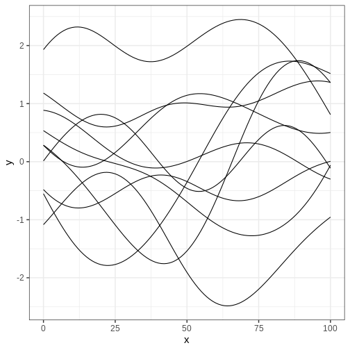
Challenge
Generate samples from the GP above with different values of \(\alpha\) and \(\lambda\) to get intuition about the role of these hyperparameters.
Implement the exponential covariance kernel defined as \(K_{exp}(x, x’) = \alpha^2 \exp{ \frac{|x - x’|}{\lambda} }\) and generate samples using this kernel. What is the qualitative difference to samples generated with squared exponential covariance?
Next, we’ll explore some examples that make use of Gaussian processes.
Example 1: Gaussian process regression
Assume we’d like to estimate the relationship between variables \(x\) and \(y\) based on the following 5 data points.
R
df6 <- data.frame(x = c(-2.76, 2.46, -1.52, -4.34, 4.54,  1),
                 y = c(-0.81, -0.85, 0.76, -0.41, -1.48,  0.2))

# Plot
p_data <- df6 %>%
  ggplot(aes(x,y)) +
  geom_point()

p_data
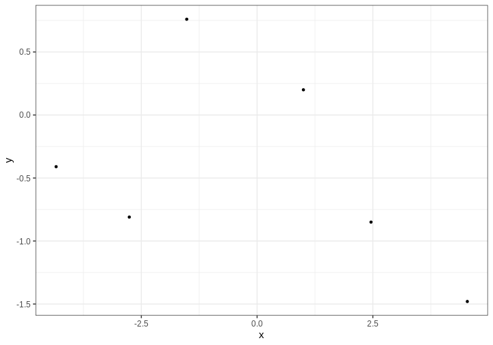
We’ll assume \(y\) are noisy
observations from some unknown function \(f(x)\) for which we’ll give a GP prior.
Because we will not recover any functional (such as polynomial) form for
\(f\), we will only learn the value of
\(f\) at separate predetermined
locations \(x\). The covariance
function needs to be computed in all those points. Let’s estimate \(f\) on a grid of points spanning the
interval (-5, 5), stored in vector x_pred:
R
x_pred <- seq(-5, 5, by = 0.1)
N_pred <- length(x_pred)
Next we’ll build the Stan program. The model structure is simple: the
model block defines the likelihood as the normal distribution with mean
\(f(x)\):
y ~ normal(f[1:N_data], sigma). Notice that this is a
vectorized statement so the mean \(y_i\) equals \(f(x_i)\) for all \(i\).
The parameter vector f contains the values of \(f\) corresponding to the data points, in
addition to the locations where we want interpolate. The covariance
function is computed in the transformed data block, where first a vector
of concatenated data and prediction locations is build. For
computational stability, it is customary to add a small value on the
diagonal of the covariance matrix. This ensures that the matrix is
positive semi-definite.
Take a moment to digest the structure of the Stan program.
STAN
data {
  // Data
  int<lower=1> N_data;
  real y[N_data];
  real x_data[N_data];

  // GP hyperparameters
  real<lower=0> alpha;
  real<lower=0> lambda;

  // Observation error
  real<lower=0> sigma;

  // Prediction points
  int<lower=1> N_pred;
  real x_pred[N_pred];
}
transformed data {
  // Number of data and prediction points
  int<lower=1> N = N_data + N_pred;

  real x[N];
  matrix[N, N] K;

  x[1:N_data] = x_data;
  x[(N_data+1):N] = x_pred;

  // Covariance function
  K = gp_exp_quad_cov(x, alpha, lambda);

  // Add nugget on diagonal for numerical stability
  for (n in 1:N) {
    K[n, n] = K[n, n] + 1e-6;
  }

}
parameters {
  vector[N] f;
}
model {
  // Likelihood
  y ~ normal(f[1:N_data], sigma);
  // GP prior
  f ~ multi_normal(rep_vector(0, N), K);
}
Let’s fit the model. We’ll use hyperparameter values \(\lambda = 1\), \(\alpha = 1\) and set the observation error standard deviation to \(\sigma = 0.1\).
R
# Fit
gp_samples <- rstan::sampling(gp_model,
                       list(N_data = nrow(df6),
                            x_data = as.array(df6$x),
                            y = as.array(df6$y),
                            lambda = 1,
                            alpha = 1,
                            sigma = 0.1,
                            N_pred = N_pred,
                            x_pred = x_pred),
                       chains = 1, iter = 1000)
OUTPUT
SAMPLING FOR MODEL 'anon_model' NOW (CHAIN 1).
Chain 1:
Chain 1: Gradient evaluation took 8.8e-05 seconds
Chain 1: 1000 transitions using 10 leapfrog steps per transition would take 0.88 seconds.
Chain 1: Adjust your expectations accordingly!
Chain 1:
Chain 1:
Chain 1: Iteration:   1 / 1000 [  0%]  (Warmup)
Chain 1: Iteration: 100 / 1000 [ 10%]  (Warmup)
Chain 1: Iteration: 200 / 1000 [ 20%]  (Warmup)
Chain 1: Iteration: 300 / 1000 [ 30%]  (Warmup)
Chain 1: Iteration: 400 / 1000 [ 40%]  (Warmup)
Chain 1: Iteration: 500 / 1000 [ 50%]  (Warmup)
Chain 1: Iteration: 501 / 1000 [ 50%]  (Sampling)
Chain 1: Iteration: 600 / 1000 [ 60%]  (Sampling)
Chain 1: Iteration: 700 / 1000 [ 70%]  (Sampling)
Chain 1: Iteration: 800 / 1000 [ 80%]  (Sampling)
Chain 1: Iteration: 900 / 1000 [ 90%]  (Sampling)
Chain 1: Iteration: 1000 / 1000 [100%]  (Sampling)
Chain 1:
Chain 1:  Elapsed Time: 32.166 seconds (Warm-up)
Chain 1:                36.453 seconds (Sampling)
Chain 1:                68.619 seconds (Total)
Chain 1:
WARNING
Warning: There were 496 transitions after warmup that exceeded the maximum treedepth. Increase max_treedepth above 10. See
https://mc-stan.org/misc/warnings.html#maximum-treedepth-exceeded
WARNING
Warning: Examine the pairs() plot to diagnose sampling problemsWARNING
Warning: The largest R-hat is 2.12, indicating chains have not mixed.
Running the chains for more iterations may help. See
https://mc-stan.org/misc/warnings.html#r-hat
WARNING
Warning: Bulk Effective Samples Size (ESS) is too low, indicating posterior means and medians may be unreliable.
Running the chains for more iterations may help. See
https://mc-stan.org/misc/warnings.html#bulk-ess
WARNING
Warning: Tail Effective Samples Size (ESS) is too low, indicating posterior variances and tail quantiles may be unreliable.
Running the chains for more iterations may help. See
https://mc-stan.org/misc/warnings.html#tail-ess
The inference takes some time (about a minute on a standard laptop) even though we only use (an insufficient) single chain and 1000 iterations. Stan also throws warnings about convergence issues. Let’s ignore these at this point, and look at the output.
R
f_samples <- rstan::extract(gp_samples, "f")[["f"]] %>%
  t %>% data.frame() %>%
  mutate(x = c(df6$x, x_pred)) # data and prediction locations

f_samples_l <- f_samples %>%
  gather(key = "sample", value = "f", -x)

p_f <- ggplot() +
  geom_line(
    data = f_samples_l,
    aes(x = x, y = f, group = sample),
    alpha = 0.05) +
  geom_point(data = df6,
             aes(x = x, y = y), color ="red")

print(p_f)
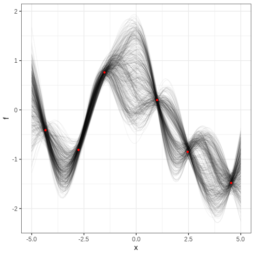
The figure contains the data points in red and samples from the posterior distribution of \(f\) in black. Each posterior sample corresponds to a function. This distribution essentially captures the model’s interpretation of the underlying trend within the data. The estimate for the trend seems plausible.
Challenge
In the figure above, where is the posterior uncertainty the highest and why? What controls the uncertainty at the locations of the data? If we made the prediction range wider, say, from -10 to 10, what would the posterior look like at the extremes?
Uncertainty grows at locations away from the data points and starts to resemble the prior. At the data locations, the uncertainty is controlled by the parameter \(\sigma\). Far from the data, the posterior would be centered around 0 and have variance \(\alpha^2\).
Cholesky parameterization
Running the previous example look a few minutes even though the amount data and number of prediction locations was modest. Scalability is a weak point of Gaussian processes but luckily there is a trick that can be used to speed up the inference and to improve convergence.
By using the Cholesky decomposition of the covariance function \(K = LL^T\), the target function \(f\) can be reparameterized as \(f = \mu + L\eta\). Now, if the random variable \(\eta\) is distributed as multivariate normal with mean 0 and identity covariance matrix, it implies that \(f \sim GP(\mu, K)\).
The Stan program below implements this parameterization. The Cholesky decomposition is performed at the end of the transformed data block and the reparameterization in the transformed parameters block. The likelihood statement is unchanged but prior is now given for \(\eta\). Other parts of the program are identical to the previous example.
STAN
data {
  // Data
  int<lower=1> N_data;
  real y[N_data];
  real x_data[N_data];

  // GP hyperparameters
  real<lower=0> alpha;
  real<lower=0> lambda;

  real<lower=0> sigma;

  // Prediction points
  int<lower=1> N_pred;
  real x_pred[N_pred];
}
transformed data {
  int<lower=1> N = N_data + N_pred;

  real x[N];
  matrix[N, N] K;
  matrix[N, N] L;

  x[1:N_data] = x_data;
  x[(N_data+1):N] = x_pred;

  // Covariance function
  K = gp_exp_quad_cov(x, alpha, lambda);

  // Add nugget on diagonal for numerical stability
  for (n in 1:N) {
    K[n, n] = K[n, n] + 1e-6;
  }

  L = cholesky_decompose(K);
}
parameters {
  vector[N] eta;
}
transformed parameters {
  // mu = (0, 0, ..., 0)
  vector[N] f = L*eta;
}
model {
  // Likelihood
  y ~ normal(f[1:N_data], sigma);
  // GP
  eta ~ normal(0, 1);
}
Let’s compile and fit this model using the same data. Fitting is completed in a few seconds with no convergence issues:
R
gp_cholesky_samples <- rstan::sampling(gp_cholesky_model,
                       list(N_data = nrow(df6),
                            x_data = as.array(df6$x),
                            y = as.array(df6$y),
                            lambda = 1,
                            alpha = 1,
                            sigma = 0.1,
                            N_pred = N_pred,
                            x_pred = x_pred),
                       chains = 1, iter = 2000,
                       refresh = 0)
Let’s examine the results. How is the posterior different from the one recovered without the Cholesky parameterization?
R
f_cholesky_samples <- rstan::extract(gp_cholesky_samples, "f")[["f"]] %>%
  t %>% data.frame() %>%
  mutate(x = c(df6$x, x_pred))

f_cholesky_samples_l <- f_cholesky_samples %>%
  gather(key = "sample", value = "f", -x)

p_cholesky_f <- ggplot() +
  geom_line(
    data = f_cholesky_samples_l,
    aes(x = x, y = f, group = sample),
    alpha = 0.05) +
  geom_point(data = df6,
             aes(x = x, y = y), color ="red")

print(p_cholesky_f)
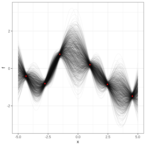
Challenge
For the previous example, compute the posterior probability for \(f(0) > 0\).
R
# Marginal posterior at x == 0
posterior_at_0 <- f_cholesky_samples_l %>%
  filter(x == 0)

mean(posterior_at_0 > 0)
OUTPUT
[1] 0.5946667Example 2: Logistic Gaussian process regression
Gaussian processes can also be used as priors in models where the relationship between the explanatory and response variables is more complex.
Consider, for example, predicting the presence of some insect species in different regions based on average annual temperature. Now the response variable \(y\) is binary with \(y=0\) and \(y=1\) corresponding to absence and presence, respectfully.
The following simulated data contains observations from 40 locations including presence/absence observations for an insect species and yearly average temperature. Plotting the data suggests there is a temperature range where the species can exists.
R
insect <- data.frame(
  x = c(1.74, 13.46, 3.69, 16.09, 8.52, 11.11, 19.32, 5.79, 11.44, 2.32, 0.67, 23.29, 14.1, 16.96, 16.29, 20.16, 12.68, 3.61, 14.22, 11.1, 8.02, 13.35, 24.48, 4.04, 21.41, 6.64, 1.36, 8.97, 17.87, 3.51, 15.68, 8.12, 1.38, 13.39, 3.01, 13.84, 5.29, 20.13, 5.57, 24.51, 3.94, 17.53, 10.62, 3.26, 19.78, 21.93, 21.47, 18.3, 15.91, 8.51),
  y = c(0, 1, 0, 1, 0, 1, 0, 0, 1, 0, 0, 0, 0, 1, 1, 0, 0, 0, 1, 0, 0, 1, 0, 0, 0, 0, 0, 1, 0, 0, 1, 0, 0, 0, 0, 1, 0, 0, 0, 0, 0, 1, 0, 0, 0, 0, 0, 1, 0, 0)
)

p <- insect %>%
  ggplot() +
  geom_point(aes(x, y))

print(p)
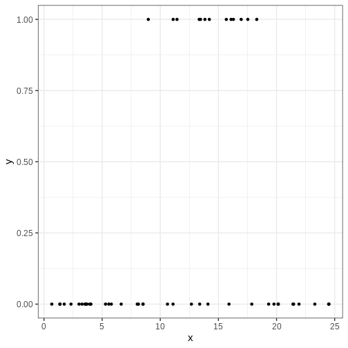
One way of modeling presence/absence data is with logistic regression:
\[ y \sim \text{Bernoulli}(\theta) \\ \theta = \frac{1}{1 + e^{-(\alpha + \beta x)}},\] where \(\alpha, \beta\) are real numbers and \(\theta\) is the probability of \(y = 1\).
However, in this standard form, the relationship between temperature and presence is monotonous: assuming \(\beta > 0\), higher temperatures imply higher probability of presence. This is in disagreement with the data and, of course, with reality. For this reason, we will modify the model so that the term \(\beta x\) is replaced with a non-parametric function \(f(x)\), that is given a GP prior. For the baseline parameter \(\alpha\), we will use a normal prior \(N(0, 10)\).
In the model block, we utilize the built-in Stan function
bernoulli_logit to write the likelihood statement. The
probability of presence as a function of temperature \(\theta\) is generated in the generated
quantities block.
STAN
data {
  // Data
  int<lower=1> N_data;
  int<lower=0, upper=1> y[N_data];
  real x_data[N_data];

  // Prediction points
  int<lower=1> N_pred;
  real x_pred[N_pred];

  // GP hyperparameters
  real<lower=0> alpha;
  real<lower=0> lambda;
}
transformed data {
  int<lower=1> N = N_data + N_pred;

  real x[N];
  matrix[N, N] K;
  matrix[N, N] L;

  x[1:N_data] = x_data;
  x[(N_data+1):N] = x_pred;

  // Covariance function
  K = gp_exp_quad_cov(x, alpha, lambda);

  // Add nugget on diagonal for numerical stability
  for (n in 1:N) {
    K[n, n] = K[n, n] + 1e-6;
  }

  L = cholesky_decompose(K);

}
parameters {
  real a;
  vector[N] eta;
}
transformed parameters {
  // mu = (0, 0, ..., 0)
  vector[N] f = L*eta;
}
model {

  // Likelihood
  y ~ bernoulli_logit(a + f[1:N_data]);
  // Priors
  a ~ normal(0, 10);
  eta ~ normal(0, 1);
}
generated quantities{
  vector[N] theta = 1 / (1 + exp(-(alpha + f)));
}
Let’s fit the model and extract the posterior summary of \(\theta\).
R
x_pred <- seq(min(insect$x), max(insect$x), length.out = 100)
N_pred <- length(x_pred)

logistic_gp_fit <- rstan::sampling(logistic_gp_model,
                                   list(N_data = nrow(insect),
                                        y = insect$y,
                                        x_data = insect$x,
                                        alpha = 1,
                                        lambda = 3,
                                        N_pred = N_pred,
                                        x_pred = x_pred),
                                   refresh = 0)

theta_summary <- rstan::summary(logistic_gp_fit, "theta")$summary %>%
  data.frame() %>%
  select(lower_2.5 = X2.5., mean, upper_97.5 = X97.5.) %>%
  mutate(x = c(insect$x, x_pred))
Then we’ll look at the posterior of \(\theta\), the probability of presence of the species and overlay it with the data. The posterior looks reasonable in the sense that the posterior of \(\theta\) is higher in the temperature range where presence was observed. However, the posterior values seem too high across the temperature range and, moreover, start veering up at the ends. Why might this be?
R
p_theta <-
  ggplot() +
  geom_ribbon(data = theta_summary,
              aes(x = x, ymin = lower_2.5, ymax = upper_97.5),
              fill = posterior_color, alpha = 0.5) +
  geom_line(data = theta_summary,
            aes(x = x, y = mean), color = posterior_color) +
  geom_point(data = insect,
             aes(x = x, y = y))

p_theta
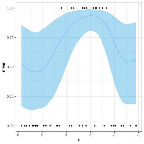
Challenge
Think of ways to modify the Stan program for the logistic GP regression so that the posterior behavior is more reasonable in the prediction range.
Let’s modify the program by setting the GP mean to a negative value and treating the length scale as a parameter.
STAN
data {
  // Data
  int<lower=1> N_data;
  int<lower=0, upper=1> y[N_data];
  real x_data[N_data];

  // Prediction points
  int<lower=1> N_pred;
  real x_pred[N_pred];

  real<lower=0> alpha;
}
transformed data {
  int<lower=1> N = N_data + N_pred;
  real x[N];
  x[1:N_data] = x_data;
  x[(N_data+1):N] = x_pred;
}
parameters {
  real a;
  vector[N] eta;
  real<lower=0> lambda;
}
transformed parameters {

  matrix[N, N] K;
  matrix[N, N] L;
  vector[N] f;

  // Covariance function
  K = gp_exp_quad_cov(x, alpha, lambda);

  // Add nugget on diagonal for numerical stability
  for (n in 1:N) {
    K[n, n] = K[n, n] + 1e-6;
  }

  L = cholesky_decompose(K);
  f = rep_vector(-3, N) + L*eta;
}
model {
  // Likelihood
  y ~ bernoulli_logit(a + f[1:N_data]);
  // Priors
  a ~ normal(0, 10);
  eta ~ normal(0, 1);
  lambda ~ gamma(2, 1);
}
generated quantities{
  vector[N] theta = 1 / (1 + exp(-(alpha + f)));
}
Refit the model and check posterior
R
logistic_gp_fit2 <- rstan::sampling(logistic_gp_model2,
                                   list(N_data = nrow(insect),
                                        y = insect$y,
                                        x_data = insect$x,
                                        alpha = 1,
                                        N_pred = N_pred,
                                        x_pred = x_pred),
                                   chains = 1)
OUTPUT
SAMPLING FOR MODEL 'anon_model' NOW (CHAIN 1).
Chain 1:
Chain 1: Gradient evaluation took 0.001306 seconds
Chain 1: 1000 transitions using 10 leapfrog steps per transition would take 13.06 seconds.
Chain 1: Adjust your expectations accordingly!
Chain 1:
Chain 1:
Chain 1: Iteration:    1 / 2000 [  0%]  (Warmup)
Chain 1: Iteration:  200 / 2000 [ 10%]  (Warmup)
Chain 1: Iteration:  400 / 2000 [ 20%]  (Warmup)
Chain 1: Iteration:  600 / 2000 [ 30%]  (Warmup)
Chain 1: Iteration:  800 / 2000 [ 40%]  (Warmup)
Chain 1: Iteration: 1000 / 2000 [ 50%]  (Warmup)
Chain 1: Iteration: 1001 / 2000 [ 50%]  (Sampling)
Chain 1: Iteration: 1200 / 2000 [ 60%]  (Sampling)
Chain 1: Iteration: 1400 / 2000 [ 70%]  (Sampling)
Chain 1: Iteration: 1600 / 2000 [ 80%]  (Sampling)
Chain 1: Iteration: 1800 / 2000 [ 90%]  (Sampling)
Chain 1: Iteration: 2000 / 2000 [100%]  (Sampling)
Chain 1:
Chain 1:  Elapsed Time: 17.53 seconds (Warm-up)
Chain 1:                17.681 seconds (Sampling)
Chain 1:                35.211 seconds (Total)
Chain 1:
R
theta_summary2 <- rstan::summary(logistic_gp_fit2, "theta")$summary %>%
  data.frame() %>%
  select(lower_2.5 = X2.5., mean, upper_97.5 = X97.5.) %>%
  mutate(x = c(insect$x, x_pred))

p_theta2 <-
  ggplot() +
  geom_ribbon(data = theta_summary2,
              aes(x = x, ymin = lower_2.5, ymax = upper_97.5),
              fill = posterior_color, alpha = 0.5) +
  geom_line(data = theta_summary2,
            aes(x = x, y = mean), color = posterior_color) +
  geom_point(data = insect,
             aes(x = x, y = y))

p_theta2
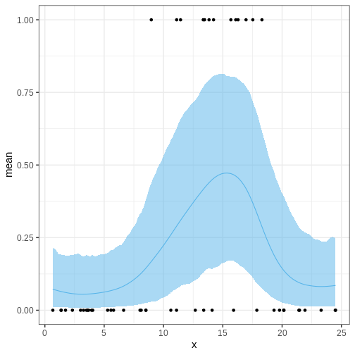
Challenge
Generate a posterior for the optimal temperature.
- GPs provide a means for non-parametric regression.
- A GP has two parameters: mean, and covariance.
- GPs can be used a part of more complex models.
Content from Stan extensions
Last updated on 2025-11-10 | Edit this page
Estimated time: 12 minutes
Overview
Questions
- Which packages take advantage of Stan and how to use them?
Objectives
- Learn to use Stan with additional R packages
In this chapter, we will introduce packages that take advantage of
Stan. The covered packages are loo, which enables
approximate Bayesian cross-validation, bayesplot, which
contains plotting tools, and brms, which allows calling
Stan using common R syntax, without having to write the Stan code.
loo
The loo package allows computing approximate
leave-one-out cross-validation (loo-cv) for models fitted with Stan. The
approximation is based on something called Pareto smoothed importance
sampling (PSIS) [1]. The package can also be used for computing WAIC and
model weights for average predictive distributions.
Example 1
We will demonstrate loo package usage on the model
comparison example studied in Episode 5. We will fit the normal and
Cauchy models on the same synthetic data, then use the tools provided in
loo to compute and compare the approximate loo-cv scores
for these two models.
To be able to utilize the package functions, we need to add a
log-likelihood computation in the Stan code, in the generated quantities
block. The object containing the log-likelihood needs to be named
log_lik so the ‘loo’ functions can find it. Below, we
demonstrate this with the two models we are comparing.
STAN
// Normal model
data {
  int<lower=0> N;
  vector[N] X;
}
parameters {
  real<lower=0> sigma;
  real mu;
}
model {
  X ~ normal(mu, sigma);

  mu ~ normal(0, 1);
  sigma ~ gamma(2, 1);
}

generated quantities {
  vector[N] X_rep;

  for(i in 1:N) {
    X_rep[i] = normal_rng(mu, sigma);
  }

  // Calculating log-likelihood for loo
  vector[N] log_lik;

  for (i in 1:N) {
  log_lik[i] = normal_lpdf(X[i] | mu, sigma);
  }
}
STAN
// Cauchy model
data {
  int<lower=0> N;
  vector[N] X;
}
parameters {
  // Scale
  real<lower=0> sigma;
  // location
  real mu;
}
model {
  // location = mu and scale = sigma
  X ~ cauchy(mu, sigma);

  mu ~ normal(0, 1);
  sigma ~ gamma(2, 1);
}
generated quantities {
  vector[N] X_rep;
  for(i in 1:N) {
    X_rep[i] = cauchy_rng(mu, sigma);
  }

  // Calculating log-likelihood for loo
  vector[N] log_lik;

  for (i in 1:N) {
  log_lik[i] = cauchy_lpdf(X[i] | mu, sigma);
  }
}
Now we can fit the models in the usual way.
R
# Fit normal model
normal_fit <- rstan::sampling(normal_model_loo,
                       list(N = N, X = df5$X),
                       refresh = 0, seed = 2024)
# Fit cauchy model
cauchy_fit <- rstan::sampling(cauchy_model_loo,
                       list(N = N, X = df5$X),
                       refresh = 0, seed = 2024)
We can now compute PSIS-LOO for both of the models with
loo::loo function. After the calling the function,
information about the fit can be viewed by printing the loo
objects.
R
# PSIS-LOO computation for normal model
normal_loo <- loo::loo(normal_fit)
WARNING
Warning: Some Pareto k diagnostic values are too high. See help('pareto-k-diagnostic') for details.R
print(normal_loo)
OUTPUT
Computed from 4000 by 88 log-likelihood matrix.

         Estimate   SE
elpd_loo   -288.8 41.6
p_loo        18.5 17.6
looic       577.7 83.3
------
MCSE of elpd_loo is NA.
MCSE and ESS estimates assume MCMC draws (r_eff in [0.8, 0.9]).

Pareto k diagnostic values:
                         Count Pct.    Min. ESS
(-Inf, 0.7]   (good)     87    98.9%   2167
   (0.7, 1]   (bad)       0     0.0%   <NA>
   (1, Inf)   (very bad)  1     1.1%   <NA>
See help('pareto-k-diagnostic') for details.
R
# PSIS-LOO computation for cauchy model
cauchy_loo <- loo::loo(cauchy_fit)
print(cauchy_loo)
OUTPUT
Computed from 4000 by 88 log-likelihood matrix.

         Estimate   SE
elpd_loo   -206.9 14.7
p_loo         2.0  0.0
looic       413.8 29.3
------
MCSE of elpd_loo is 0.0.
MCSE and ESS estimates assume MCMC draws (r_eff in [0.7, 0.8]).

All Pareto k estimates are good (k < 0.7).
See help('pareto-k-diagnostic') for details.
Running print returns \(\widehat{\text{elpd}}_{\text{loo}}\)
(expected log pointwise predictive density), \(\hat{p}_{loo}\) (estimated number of
parameters) and \(\text{looic}\) (LOO
information criterion) values and their standard errors. It also returns
a table with the Pareto \(k\)
diagnostic values, which are used to asses the reliability of the
estimates. Values below 1 are required for reliable PSIS estimates.
Model comparison can be done by using the
loo::loo_compare function on the loo objects.
The comparison is based on the models’ elpd values.
R
# Comparing models based on loo
loo::loo_compare(normal_loo, cauchy_loo)
OUTPUT
       elpd_diff se_diff
model2   0.0       0.0
model1 -81.9      36.2
The comparison shows that the elpd difference is larger than the standard error, indicating that the cauchy model is expected to have better predictive performance than the normal model. This is in line with what we saw in chapter 5: the Cauchy distribution is a superior model for the data.
Challenge
loo can also be used to compute WAIC for Bayesian
models. Calculate WAIC for the two models and then compare them.
First we need to extract the log-likelihood values from the fitted model object.
R
# Extracting loglik
normal_loglik <- loo::extract_log_lik(normal_fit)
cauchy_loglik <- loo::extract_log_lik(cauchy_fit)

# Computing WAIC for the models
normal_waic <- loo::waic(normal_loglik)
WARNING
Warning:
1 (1.1%) p_waic estimates greater than 0.4. We recommend trying loo instead.
R
print(normal_waic)
OUTPUT
Computed from 4000 by 88 log-likelihood matrix.

          Estimate   SE
elpd_waic   -290.0 42.8
p_waic        19.7 18.8
waic         580.1 85.6

1 (1.1%) p_waic estimates greater than 0.4. We recommend trying loo instead.
R
cauchy_waic <- loo::waic(cauchy_loglik)
print(cauchy_waic)
OUTPUT
Computed from 4000 by 88 log-likelihood matrix.

          Estimate   SE
elpd_waic   -206.9 14.7
p_waic         2.0  0.0
waic         413.8 29.3
Computing WAIC for the model return values for \(\widehat{\text{eldp}}_{\text{WAIC}}\), \(\hat{p}_{\text{WAIC}}\) and \(\widehat{\text{WAIC}}\). Models can be compared based on WAIC using the same function as with PSIS-LOO.
R
# Comparing models based on WAIC
loo::loo_compare(normal_waic, cauchy_waic)
OUTPUT
       elpd_diff se_diff
model2   0.0       0.0
model1 -83.1      37.4
bayesplot
Next, we will look at the the bayesplot R package. The
package provides a library of plotting functions for fitted Stan models.
The created plots are ggplot objects, meaning that the
plots can be customized with the functions from ggplot2
package. The package enables plotting posterior draws, visual MCMC
diagnostics and graphical posterior and prior predictive checking. The
functions of the package also work with model fit with the popular
packages brms and rstanarm.
Example 1 continued
We will demonstrate using bayesplot with the Cauchy
model used in the first example. First, we need to extract the posterior
draws. Then, we will plot uncertainty intervals for \(\mu\) and \(\sigma\).
R
# Extracting draws
cauchy_draws <- as.array(cauchy_fit)

# Plotting uncertainty intervals
bayesplot::mcmc_intervals(cauchy_draws, pars = c("mu", "sigma"))
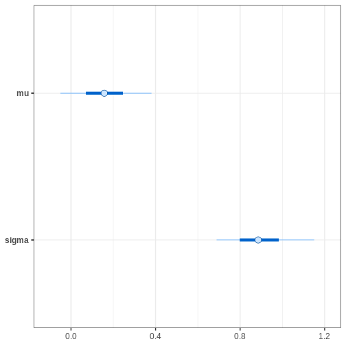
Alternatively, we can plot the (marginal) posterior sample histograms or densities with credible intervals as shaded areas as follows:
R
# Plotting estimated density curves
bayesplot::mcmc_areas(cauchy_draws, pars = c("mu", "sigma"),
                      prob = 0.95,
                      point_est = "mean")
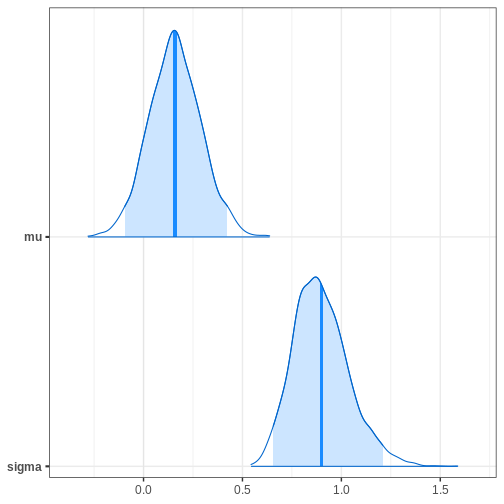
R
# Plotting histogram
bayesplot::mcmc_hist(cauchy_draws, pars = c("mu", "sigma"))
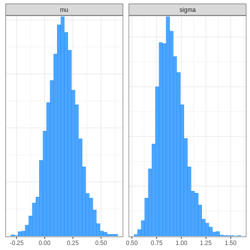
bayesplot also provides functions for assessing MCMC
convergence and visualizing fit diagnostics. For example, we can
generate trace plots for the chains:
R
# Plotting trace plot
bayesplot::mcmc_trace(cauchy_draws, pars = c("mu", "sigma"),
                      facet_args = list(ncol = 1))
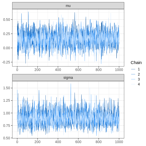
Challenge
Perform a graphical posterior predictive checks with
bayesplot. Using the Cauchy model fit generated above, plot
the density of \(X_{rep}\) samples
overlaid with the density of \(X\).
Alternatively, you can plot the corresponding histograms.
R
# Extracting replicates and getting a subset
set.seed(2024)
X_rep <- rstan::extract(cauchy_fit, "X_rep")[[1]] %>%
  data.frame() %>%
    mutate(sample = 1:nrow(.))

N_rep <- 9

X_rep_sub <- X_rep %>% filter(sample %in%
                                sample(X_rep$sample,
                                       N_rep,
                                       replace = FALSE))
X_rep_sub <- X_rep_sub[, -89] %>%
  as.matrix()
R
# Plot density
# Limit x range for better illustration
bayesplot::ppc_dens_overlay(y = df5$X, yrep = X_rep_sub) + xlim(-25, 50)
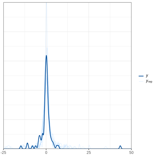
R
# Plot histograms
bayesplot::ppc_hist(y = df5$X, yrep = X_rep_sub) + xlim(-25,50)
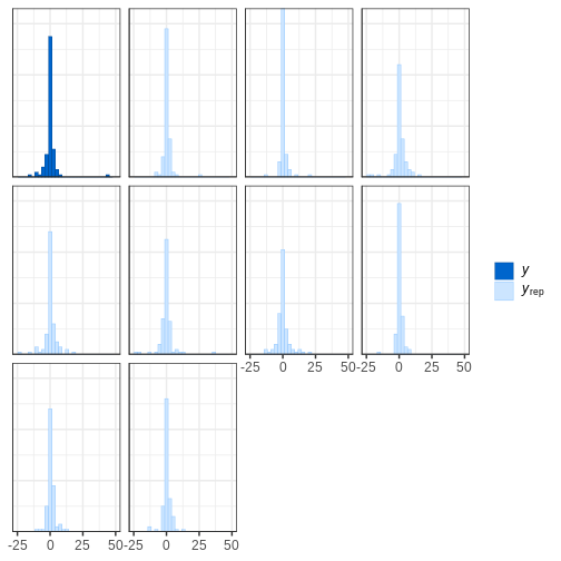
brms R package
We will now introduce the brms R package. The package
allows fitting probabilistic generalized (non-)linear models with Stan.
A large range of distributions and link functions are supported, in
addition to multilevel structure. Moreover, several built-in functions
are available for priors.
Models are specified using familiar R formula syntax, input into an R function which compiles and calls the Stan model in the backend.
The package also provides tools for evaluating the fit and MCMC
convergence. These tools, in turn, use functions from the
loo and bayesplot packages, that is, many of
the same tools we covered earlier in this Episode.
Next, we will demonstrate usage of the package with two different examples.
Example 2: Survival modeling
In this example, we will demonstrate fitting a Cox proportional
hazard model with brms. However, first, we will briefly
describe and model and idea in survival modeling.
The Cox model is a standard approach used in survival modeling, in which the outcome of interest is the time to some event. A common application is medical studies where patients are followed in time until an event (e.g. death) or until censoring. A subject is censored if the event doesn’t occur during the follow-up.
An important ingredient in survival modeling is the hazard function, representing the instantaneous risk for an event at time \(t\), defined as \(\lambda(t)=\text{lim}_{h \to 0+} \frac{1}{h}P(t \le T<t+h|T\ge t)\). In the Cox model, the hazard function is of the form \(\lambda(t_i,Z_i,\theta)=\lambda_0(t_i)\text{exp}(\beta^\prime Z_i)\).
The baseline hazard function \(\lambda_0(t_i)\) represents the hazard when the covariates are set to their baselines, and is the same for each subject \(i\). Commonly, the functional form the baseline hazard is not specified. The second part of the hazard function contains subject-specific covariates, \(\text{exp}(\beta^\prime Z_i)\).
The exponentials of the effects \(\beta\) are called hazard ratios, which measure the hazard in one group against the hazard in another group.
When fitting the Cox model, brms uses M-splines for the
baseline hazard. Splines are functions built from piecewise-defined
polynomials. In other words, the baseline hazard is a combination of
several different polynomial functions. M-splines are non-negative
spline functions, which is important for reasons we omit. However,
hopefully, the reader can appreciate the simplicity of the upcoming
brms function call.
Before fitting the model, we will take a look at the
lung dataset from the survival R package,
which we will be analyzing below. The dataset consists of survival times
of patients with advanced lung cancer including some clinical
covariates.
R
# Get data
lung <- survival::lung

# Take a peek
head(lung)
OUTPUT
  inst time status age sex ph.ecog ph.karno pat.karno meal.cal wt.loss
1    3  306      2  74   1       1       90       100     1175      NA
2    3  455      2  68   1       0       90        90     1225      15
3    3 1010      1  56   1       0       90        90       NA      15
4    5  210      2  57   1       1       90        60     1150      11
5    1  883      2  60   1       0      100        90       NA       0
6   12 1022      1  74   1       1       50        80      513       0
The variable status denotes if an event (death) was
observed or if the subject was censored. We will use three covariates:
age, sex and ph.karno. The
variable ph.karno describes how well a patient can perform
daily activities rated by a physician. We will split the variable into
two categories “high” and “low.”
Cox model can be fit with brms::brm() function by
specifying family = brmsfamily("cox"). Censored data points
are indicated with the cens(1 - status) argument. We will
use a standard \(\text{Normal}(0, 10)\)
prior for the population-level effects, with the argument
prior(normal(0,10), class = b). The option
class = b sets the prior for all population-level
effects.
R
# Let's change status coding from 2/1 to 1/0
lung$status <- lung$status - 1

# Remove observations with NA ph.karno
lung <- lung[!is.na(lung$ph.karno),]

# Creating new variable for ph.karno status
lung$ph.karno_status <- cut(lung$ph.karno,
                            breaks = c(0, 70, 100),
                            labels = c("low", "high"))

# Fitting the model
fit_cox <- brms::brm(time | cens(1 - status) ~ sex + age + ph.karno_status,
             data = lung, family = brmsfamily("cox"), seed = 2024,
             silent = 2, refresh = 0, cores = 4,
             prior = prior(normal(0,10), class = b))
# Summary of the fit
summary(fit_cox)
OUTPUT
 Family: cox
  Links: mu = log
Formula: time | cens(1 - status) ~ sex + age + ph.karno_status
   Data: lung (Number of observations: 227)
  Draws: 4 chains, each with iter = 2000; warmup = 1000; thin = 1;
         total post-warmup draws = 4000

Regression Coefficients:
                    Estimate Est.Error l-95% CI u-95% CI Rhat Bulk_ESS Tail_ESS
Intercept               1.27      0.68    -0.11     2.57 1.00     4304     2666
sex                    -0.50      0.16    -0.83    -0.19 1.00     4768     2842
age                     0.01      0.01    -0.01     0.03 1.00     4607     2784
ph.karno_statushigh    -0.36      0.18    -0.70    -0.02 1.00     4471     2616

Draws were sampled using sampling(NUTS). For each parameter, Bulk_ESS
and Tail_ESS are effective sample size measures, and Rhat is the potential
scale reduction factor on split chains (at convergence, Rhat = 1).
The summary output of the brms fit prints coefficient
estimates, and also returns Rhat, Bulk_ESS and Tail_ESS values, which
can be used to assess the convergence of the model.
It is important to notice that the coefficients are the log hazard
ratios, which means we still need to exponentiate them. The
bayesplot::mcmc_intervals() function allows transforming
the parameters before plotting with transform = "exp"
argument.
R
# Get hazard values
sum_cox <- summary(fit_cox)
exp(sum_cox$fixed[,1:4])
OUTPUT
                     Estimate Est.Error  l-95% CI   u-95% CI
Intercept           3.5576154  1.970680 0.8962140 13.1193479
sex                 0.6044998  1.179035 0.4369700  0.8279120
age                 1.0130229  1.009435 0.9945742  1.0318059
ph.karno_statushigh 0.6956990  1.193047 0.4959062  0.9847118
R
# Credible intervals
bayesplot::mcmc_intervals(fit_cox,
                          pars = c("b_sex", "b_age", "b_ph.karno_statushigh"),
                          transform = "exp")
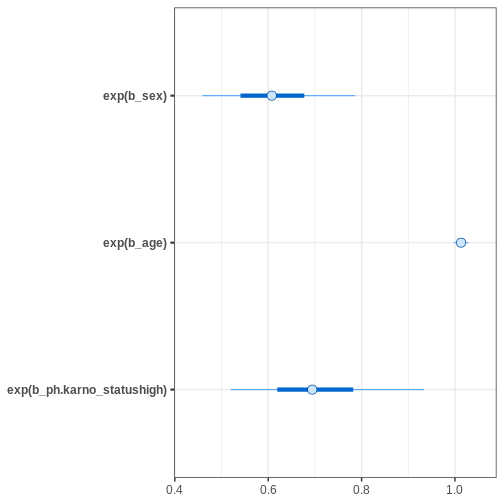
Based on the estimates, it seems that age has only a minor effect on
the hazard. Female sex and being “high” in ph.karno imply
smaller hazards, meaning that these factors are protective.
After fitting the model, we can print information about the priors
used with the function brms::get_prior.
R
# Get priors for the cox model
brms::get_prior(fit_cox)
OUTPUT
                  prior     class                coef group resp dpar nlpar lb
          normal(0, 10)         b
          normal(0, 10)         b                 age
          normal(0, 10)         b ph.karno_statushigh
          normal(0, 10)         b                 sex
 student_t(3, 5.6, 2.5) Intercept
           dirichlet(1)     sbhaz
 ub       source
            user
    (vectorized)
    (vectorized)
    (vectorized)
         default
         default
The population-level effects have the normal prior we specified. In
brms, the default prior for the intercept is Student’s
t-distribution with three degrees of freedom. The Stan program
brms ran under the hood can be printed with the
brms::stancode function.
R
# Print the Stan code
brms::stancode(fit_cox)
OUTPUT
// generated with brms 2.22.0
functions {
  /* distribution functions of the Cox proportional hazards model
   * parameterize hazard(t) = baseline(t) * mu
   * so that higher values of 'mu' imply lower survival times
   * Args:
   *   y: the response value; currently ignored as the relevant
   *     information is passed via 'bhaz' and 'cbhaz'
   *   mu: positive location parameter
   *   bhaz: baseline hazard
   *   cbhaz: cumulative baseline hazard
   */
  real cox_lhaz(real y, real mu, real bhaz, real cbhaz) {
    return log(bhaz) + log(mu);
  }
  vector cox_lhaz(vector y, vector mu, vector bhaz, vector cbhaz) {
    return log(bhaz) + log(mu);
  }

  // equivalent to the log survival function
  real cox_lccdf(real y, real mu, real bhaz, real cbhaz) {
    return - cbhaz * mu;
  }
  real cox_lccdf(vector y, vector mu, vector bhaz, vector cbhaz) {
    return - dot_product(cbhaz, mu);
  }

  real cox_lcdf(real y, real mu, real bhaz, real cbhaz) {
    return log1m_exp(cox_lccdf(y | mu, bhaz, cbhaz));
  }
  real cox_lcdf(vector y, vector mu, vector bhaz, vector cbhaz) {
    return sum(log1m_exp(- cbhaz .* mu));
  }

  real cox_lpdf(real y, real mu, real bhaz, real cbhaz) {
    return cox_lhaz(y, mu, bhaz, cbhaz) + cox_lccdf(y | mu, bhaz, cbhaz);
  }
  real cox_lpdf(vector y, vector mu, vector bhaz, vector cbhaz) {
    return sum(cox_lhaz(y, mu, bhaz, cbhaz)) + cox_lccdf(y | mu, bhaz, cbhaz);
  }

  // Distribution functions of the Cox model in log parameterization
  real cox_log_lhaz(real y, real log_mu, real bhaz, real cbhaz) {
    return log(bhaz) + log_mu;
  }
  vector cox_log_lhaz(vector y, vector log_mu, vector bhaz, vector cbhaz) {
    return log(bhaz) + log_mu;
  }

  real cox_log_lccdf(real y, real log_mu, real bhaz, real cbhaz) {
    return - cbhaz * exp(log_mu);
  }
  real cox_log_lccdf(vector y, vector log_mu, vector bhaz, vector cbhaz) {
    return - dot_product(cbhaz, exp(log_mu));
  }

  real cox_log_lcdf(real y, real log_mu, real bhaz, real cbhaz) {
    return log1m_exp(cox_log_lccdf(y | log_mu, bhaz, cbhaz));
  }
  real cox_log_lcdf(vector y, vector log_mu, vector bhaz, vector cbhaz) {
    return sum(log1m_exp(- cbhaz .* exp(log_mu)));
  }

  real cox_log_lpdf(real y, real log_mu, real bhaz, real cbhaz) {
    return cox_log_lhaz(y, log_mu, bhaz, cbhaz) +
           cox_log_lccdf(y | log_mu, bhaz, cbhaz);
  }
  real cox_log_lpdf(vector y, vector log_mu, vector bhaz, vector cbhaz) {
    return sum(cox_log_lhaz(y, log_mu, bhaz, cbhaz)) +
           cox_log_lccdf(y | log_mu, bhaz, cbhaz);
  }
}
data {
  int<lower=1> N;  // total number of observations
  vector[N] Y;  // response variable
  // censoring indicator: 0 = event, 1 = right, -1 = left, 2 = interval censored
  array[N] int<lower=-1,upper=2> cens;
  int<lower=1> K;  // number of population-level effects
  matrix[N, K] X;  // population-level design matrix
  int<lower=1> Kc;  // number of population-level effects after centering
  // data for flexible baseline functions
  int Kbhaz;  // number of basis functions
  // design matrix of the baseline function
  matrix[N, Kbhaz] Zbhaz;
  // design matrix of the cumulative baseline function
  matrix[N, Kbhaz] Zcbhaz;
  // a-priori concentration vector of baseline coefficients
  vector<lower=0>[Kbhaz] con_sbhaz;
  int prior_only;  // should the likelihood be ignored?
}
transformed data {
  // indices of censored data
  int Nevent = 0;
  int Nrcens = 0;
  int Nlcens = 0;
  array[N] int Jevent;
  array[N] int Jrcens;
  array[N] int Jlcens;
  matrix[N, Kc] Xc;  // centered version of X without an intercept
  vector[Kc] means_X;  // column means of X before centering
  // collect indices of censored data
  for (n in 1:N) {
    if (cens[n] == 0) {
      Nevent += 1;
      Jevent[Nevent] = n;
    } else if (cens[n] == 1) {
      Nrcens += 1;
      Jrcens[Nrcens] = n;
    } else if (cens[n] == -1) {
      Nlcens += 1;
      Jlcens[Nlcens] = n;
    }
  }
  for (i in 2:K) {
    means_X[i - 1] = mean(X[, i]);
    Xc[, i - 1] = X[, i] - means_X[i - 1];
  }
}
parameters {
  vector[Kc] b;  // regression coefficients
  real Intercept;  // temporary intercept for centered predictors
  // baseline hazard coefficients
  simplex[Kbhaz] sbhaz;
}
transformed parameters {
  real lprior = 0;  // prior contributions to the log posterior
  lprior += normal_lpdf(b | 0, 10);
  lprior += student_t_lpdf(Intercept | 3, 5.6, 2.5);
  lprior += dirichlet_lpdf(sbhaz | con_sbhaz);
}
model {
  // likelihood including constants
  if (!prior_only) {
    // compute values of baseline function
    vector[N] bhaz = Zbhaz * sbhaz;
    // compute values of cumulative baseline function
    vector[N] cbhaz = Zcbhaz * sbhaz;
    // initialize linear predictor term
    vector[N] mu = rep_vector(0.0, N);
    mu += Intercept + Xc * b;
    // vectorized log-likelihood contributions of censored data
    target += cox_log_lpdf(Y[Jevent[1:Nevent]] | mu[Jevent[1:Nevent]], bhaz[Jevent[1:Nevent]], cbhaz[Jevent[1:Nevent]]);
    target += cox_log_lccdf(Y[Jrcens[1:Nrcens]] | mu[Jrcens[1:Nrcens]], bhaz[Jrcens[1:Nrcens]], cbhaz[Jrcens[1:Nrcens]]);
    target += cox_log_lcdf(Y[Jlcens[1:Nlcens]] | mu[Jlcens[1:Nlcens]], bhaz[Jlcens[1:Nlcens]], cbhaz[Jlcens[1:Nlcens]]);
  }
  // priors including constants
  target += lprior;
}
generated quantities {
  // actual population-level intercept
  real b_Intercept = Intercept - dot_product(means_X, b);
}
Example 3: Hierarchical binomial model
We will now demonstrate one of the key focuses of brms,
fitting hierarchical models. The syntax for specifying hierarchical
models is similar as in the lme4 package, which is used to
fit frequentist multilevel models in R.
For this example, we will be using is the VerbAgg data
from lme4 package. The data consist of item responses to a
questionnaire on verbal aggression.
R
# Get data
VerbAgg <- lme4::VerbAgg

head(VerbAgg)
OUTPUT
  Anger Gender        item    resp id btype  situ mode r2
1    20      M S1WantCurse      no  1 curse other want  N
2    11      M S1WantCurse      no  2 curse other want  N
3    17      F S1WantCurse perhaps  3 curse other want  Y
4    21      F S1WantCurse perhaps  4 curse other want  Y
5    17      F S1WantCurse perhaps  5 curse other want  Y
6    21      F S1WantCurse     yes  6 curse other want  Y
We will estimate population-level effects for Anger, Gender, btype
and situ, and includea group-level intercept for id. The variable of
interest is the binary r2, which contains the response to an question in
the questionnaire. We will use \(\text{Normal}(0, 10)\) as the prior for all
the population-level effects. For the standard deviation of group-level
effect we will set a (half-)\(\text{Cauchy}(0,
5)\) prior. By default, brms uses half-Student’s
t-distribution with three degrees of freedom for standard deviation
parameters. The group-level intercept for variable id is specified with
the argument (1|id). Let’s now fit the model.
R
# Change coding for r2
VerbAgg <- VerbAgg %>%
  mutate(r2 = ifelse(r2 == "N", 0, 1))
# Fit model
fit_hier <- brms::brm(r2 ~ Anger + Gender + btype + situ + (1|id),
                      family = bernoulli,
                      data = VerbAgg,
                      seed = 2024, cores = 4, silent = 2, refresh = 0,
                      prior = prior(normal(0, 10), class = b) +
                        prior(cauchy(0,5), class = sd))
# Summary
summary(fit_hier)
OUTPUT
 Family: bernoulli
  Links: mu = logit
Formula: r2 ~ Anger + Gender + btype + situ + (1 | id)
   Data: VerbAgg (Number of observations: 7584)
  Draws: 4 chains, each with iter = 2000; warmup = 1000; thin = 1;
         total post-warmup draws = 4000

Multilevel Hyperparameters:
~id (Number of levels: 316)
              Estimate Est.Error l-95% CI u-95% CI Rhat Bulk_ESS Tail_ESS
sd(Intercept)     1.30      0.07     1.17     1.43 1.00     1086     1687

Regression Coefficients:
           Estimate Est.Error l-95% CI u-95% CI Rhat Bulk_ESS Tail_ESS
Intercept      0.21      0.34    -0.49     0.87 1.01      637     1035
Anger          0.05      0.02     0.02     0.09 1.01      664     1026
GenderM        0.31      0.19    -0.05     0.68 1.00      580     1257
btypescold    -1.03      0.07    -1.17    -0.90 1.00     4963     3254
btypeshout    -2.00      0.07    -2.14    -1.85 1.00     4867     3286
situself      -1.01      0.06    -1.12    -0.89 1.00     5877     3022

Draws were sampled using sampling(NUTS). For each parameter, Bulk_ESS
and Tail_ESS are effective sample size measures, and Rhat is the potential
scale reduction factor on split chains (at convergence, Rhat = 1).
The conditional effects of the predictors can easily be plotted with
the function brms::conditional_effects.
R
# Conditional effects
plots <- plot(conditional_effects(fit_hier), plot = FALSE)
cowplot::plot_grid(plots[[1]], plots[[2]], plots[[3]], plots[[4]])
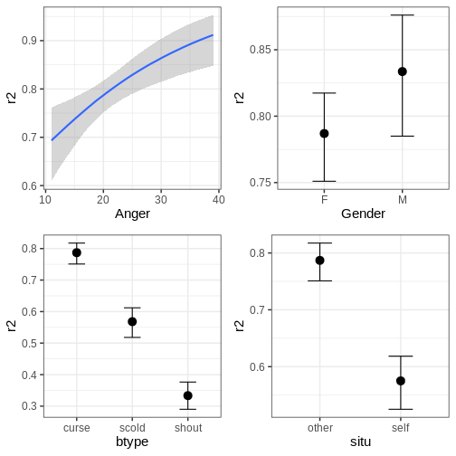
The function can also plot variable interactions. Let’s plot the conditional effect for interaction between Anger and btype.
R
# Plot conditional effect for interaction of Anger and btype
plot(conditional_effects(fit_hier, effects = "Anger:btype"))
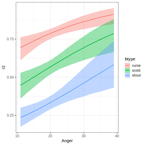
Let us now do a slight alteration in model and add another
group-level intercept for the item variable. The priors are same as in
the first model. The update function can be used to modify
the formula without writing it anew in its entirety.
R
# Update model
fit_hier2 <- update(fit_hier, formula. = ~ . + (1|item), newdata = VerbAgg, seed = 2024,
                    cores = 4, silent = 2, refresh = 0)
# Summary
summary(fit_hier2)
OUTPUT
 Family: bernoulli
  Links: mu = logit
Formula: r2 ~ Anger + Gender + btype + situ + (1 | id) + (1 | item)
   Data: VerbAgg (Number of observations: 7584)
  Draws: 4 chains, each with iter = 2000; warmup = 1000; thin = 1;
         total post-warmup draws = 4000

Multilevel Hyperparameters:
~id (Number of levels: 316)
              Estimate Est.Error l-95% CI u-95% CI Rhat Bulk_ESS Tail_ESS
sd(Intercept)     1.36      0.07     1.23     1.51 1.00     1347     1922

~item (Number of levels: 24)
              Estimate Est.Error l-95% CI u-95% CI Rhat Bulk_ESS Tail_ESS
sd(Intercept)     0.59      0.11     0.42     0.84 1.00     1404     2252

Regression Coefficients:
           Estimate Est.Error l-95% CI u-95% CI Rhat Bulk_ESS Tail_ESS
Intercept      0.18      0.44    -0.65     1.05 1.01      831     1522
Anger          0.06      0.02     0.02     0.09 1.00      801     1568
GenderM        0.32      0.20    -0.07     0.72 1.00      847     1333
btypescold    -1.06      0.30    -1.63    -0.43 1.00     1191     1561
btypeshout    -2.11      0.30    -2.71    -1.52 1.00     1284     1889
situself      -1.05      0.25    -1.54    -0.55 1.00     1156     1828

Draws were sampled using sampling(NUTS). For each parameter, Bulk_ESS
and Tail_ESS are effective sample size measures, and Rhat is the potential
scale reduction factor on split chains (at convergence, Rhat = 1).
Another useful aspect of update is that it allows
resampling from the model without having to recompile the model, for
example, using different number of iterations. However, changes to the
model itself require recompilation.
To end this section, let’s compare the two models by using
brms::loo(). This works in the same way as the
loo::loo_compare.
R
# Compare models
brms::loo(fit_hier, fit_hier2)
OUTPUT
Output of model 'fit_hier':

Computed from 4000 by 7584 log-likelihood matrix.

         Estimate   SE
elpd_loo  -4004.9 42.9
p_loo       268.0  3.7
looic      8009.7 85.8
------
MCSE of elpd_loo is 0.2.
MCSE and ESS estimates assume MCMC draws (r_eff in [1.1, 2.2]).

All Pareto k estimates are good (k < 0.7).
See help('pareto-k-diagnostic') for details.

Output of model 'fit_hier2':

Computed from 4000 by 7584 log-likelihood matrix.

         Estimate   SE
elpd_loo  -3866.9 43.9
p_loo       287.0  4.1
looic      7733.8 87.8
------
MCSE of elpd_loo is 0.2.
MCSE and ESS estimates assume MCMC draws (r_eff in [1.1, 2.6]).

All Pareto k estimates are good (k < 0.7).
See help('pareto-k-diagnostic') for details.

Model comparisons:
          elpd_diff se_diff
fit_hier2    0.0       0.0
fit_hier  -138.0      16.2
Based on the output, the second model provides a superior fit compared to the first model.
Challenge
Experiment with different priors for the model. How much does the chosen prior affect the results? Is there a big difference between a flat and the weakly informative prior used above?
Other packages built on Stan
In addition to the ones covered here, there are several other
packages that take advantage of Stan. Here we will briefly introduce
some of them. CmdStanR is a
lightweight command-line-based interface for Stan and provides and
alternative for rstan. rstanarm emulates the model
fitting R functions using Stan. The package can do lot of the same
things as brms, but they do have differences, for example
rstanarm models come pre-compiled while brms
compiles the models when called.
shinystan uses Shiny and
provides user with interactive, customizable visual and numerical
summaries of model parameters and convergence diagnostics. projpred performs projection
predictive variable selection for various models. The package works with
models from brms and rstanarm. posterior provides tools for
manipulating posterior draws, and contains methods for common
operations, such as, subsetting and binding, and producing posterior
summaries, and diagnostics.
- There are several R packages that provide more user-friendly ways of using Stan.
-
brmspackage can be used to fit a vast array of different Bayesian models. -
bayesplotpackage is a library for various plotting tools. - Approximate leave-one-out cross-validation can be performed with the
loopackage.
Reading
References
- [1] A. Vehtari et al., Pareto Smoothed Importance Sampling, Journal of Machine Learning Research 25 (2024) 1-58.
Content from Exercises
Last updated on 2025-11-10 | Edit this page
Estimated time: 12 minutes
Overview
Questions
- How can I get routine in probabilistic programming?
Objectives
The purpose of this Episode is to provide material for practicing probabilistic programming. The exercises are listed under the Episode they approximately refer to.
1. Basics
1.1 Grid approximation: normal model with unknown mean
Generate 1000 data points from the normal model. Use a randomly generated mean parameter, \(\mu \sim N(0,1)\) and set the standard deviation \(\sigma=1\).
The grid approximation for this model was introduced in Episode XX but the implementation doesn’t work for the generated data. Locate the source of error and make the necessary modifications to get the program working.
Plot the posterior of \(\mu\).
1.2 Grid approximation: Gamma-Poisson
The Gamma-Poisson model can be stated as:
\[y_i \sim \text{Pois}(\lambda) \\ \lambda \sim \Gamma(1, 1), \]
where \(y_i\) are non-negative data points, and Pois is the Poisson distribution with rate parameter \(\lambda > 0\). Implement a grid approximation for this model.
Apparently (https://en.wikipedia.org/wiki/Poisson_distribution), the number of chewing gum on a sidewalk tile is approximately Poisson distributed.
Estimate the average number of gum on a Reykjavik side walk tile (lambda), using the data
R
y <- c(2,7,4,3,5,2,7,5,5,5)
1.3 Less data means bigger prior effect
Show that as the amount of available data increases, the effect of the prior decreases.
Instructions:
- Simulate a series of coin tosses:
- Generate \(p \sim \text{Uniform}(0, 1)\).
- Simulate a sequence of 50 tosses with Pr(heads) = p.
- Fit the grid approximation using the first 1, 5, 10, 15,…, 50
tosses.
- Use a Beta prior for p.
- Compare the posteriors the prior.
1.4 Grid approximation: for a normal model with unknown mean and standard deviation
The following data is a collection of daily milk yield (in liters) for dairy cows.
R
X <- c(30.25, 34.98, 29.66, 20.14, 23.92, 38.61, 36.89, 34.68, 25.83, 29.93)
Using the grid approximation for the normal model, estimate the average daily yield \(\mu\).
Use some non-uniform priors.
Plot the marginal posterior for \(\mu\) and compute the 90% credible interval for the marginal.
What is the probability that the average daily milk yield is more than 30 liters?
1.5 Sampling the Gamma
Let’s model the following observations X with the exponential likelihood, \(\text{Exp}(\lambda)\):
R
X <-  c(0.166, 1.08, 1.875, 0.413, 1.369, 0.463, 0.735,
       0.24, 0.774, 1.09, 0.463, 0.916, 0.225,
        0.889, 0.051, 0.688, 0.119, 0.078, 1.624, 0.553, 0.523,
       0.644, 0.284, 1.744, 1.468)
If we use a \(\Gamma(2, 1)\) prior, the posterior distribution can be shown to be
\(p(\lambda | X) = \Gamma(2 + n, 1 + X_1 + X_2 + ... + X_n),\)
where \(n\) is the number of observations.
Generate 5000 samples from the posterior and compute 1. the posterior mean and mode 2. the 50% and 95% credible intervals 3. the probabilities \(Pr(\lambda > 1), Pr( 1 < \lambda < 1.5), Pr(\lambda < 1 \text{ or } \lambda > 1.5)\)
1.6 Grid approximation: Cauchy distribution
(Emulated from BDA3: p59. Ex.11)
Suppose y1,…,y5 are independent samples from a Cauchy distribution with scale 1 and unknown location \(\theta\). Given the observations \((y_1, . . . , y_5) = (43, 44, 45, 46.5, 47.5)\):
- Compute the unnormalized posterior density function, \(p(\theta)p(y|\theta)\), on a grid of points \(\theta = 0, 1/m , 2/m ,..., 100\), for some large integer \(m\). Using the grid approximation, compute and plot the normalized posterior density function as a function of \(\theta\). Assume a uniform prior for over [0, 100].
- Generate 1000 samples of \(\theta\) from the posterior and plot a histogram of the samples.
- Use each of the samples generated in b) to generate a new data point \(y_6\) from the likelihood function and plot a histogram of these draws.
1.7 Sampling the Normal
The posterior for the normal model with unknown \(\mu\) and \(\sigma\) can be sampled as follows (BDA3:p.65):
- Sample the variance from \(\sigma^2 \sim Inv-\chi^2(n-1, \text{Var}(X))\)
- Sample the mean from \(\mu | \sigma^2 ~ N(\bar{X}, \frac{\sigma^2}{n})\)
Here \(\bar{X}\) is the mean of the data points \(X = \{X_1, X_2, ..., X_n\}\).
- Generate 5000 samples from the posterior using the data
R
X <- c(21.1, 20.8, 21.9, 20.5, 18.7, 24.1, 18.6, 15.4, 16.9, 20.8)
- Compute the posterior for the coefficient of variation \(CV = \frac{\sigma}{\mu}\).
- Generate samples for an unseen data point \(\tilde{X}\).
- Compare the distribution in c) to one generated using only the MAP estimate. Is there a discrepancy and why?
1.8 HPDI
Another approach to summarizing the posterior is to compute the shortest interval that contains \(p\%\) of the posterior. Such interval is called highest posterior density interval (HPDI).
Write a function that returns the highest posterior density interval, given a set of posterior samples.
Assume that the analytical form of a posterior is known to be Gamma(3, 20). Generate samples from this distribution and compute the 90% HPDI. Compare it to the 90% credible interval.
Hint: If you sort the posterior samples in order, each set of n consecutive samples contains \(100 \cdot \frac{n}{N} \%\) of the posterior, where \(N\) is the total number of samples.
2. Stan
2.1 Gamma-Poisson model
The Gamma-Poisson model can be stated as:
\[y_i \sim \text{Pois}(\lambda) \\ \lambda \sim \Gamma(1, 1), \]
where \(y_i\) are non-negative data points, and Pois is the Poisson distribution with rate parameter \(\lambda > 0\).
Implement the model in Stan. Do it so that the parameter beta is input as part of data. Heuristically, what effect does altering beta have on the prior shape?
Fit the model using the data
R
y <- c(2,7,4,3,5,2,7,5,5,5)
Compute the MAP, mean and 90% CIs and include them in a figure with a histogram of posterior samples.
2.2 Dice
Write a Stan program that implements the following statistical model:
\[y \sim \text{categorial}(\theta) \\ \theta \sim \text{Dir}(1, 1, ..., 1), \]
where \(\theta\) is a 6-dimensional probability vector and Dir is the Dirichlet distribution.
Use the program to assess the fairness of a 6 sided dice. In other words, estimate the probabilities of each side on a roll using the following data.
R
X <- c(3, 2, 6, 3, 6, 2, 5, 6, 5, 6, 4, 1, 4, 2, 5, 4, 6, 6, 5, 4, 1, 3, 3, 4, 2, 3, 4, 4, 4, 1, 1, 3, 4, 4, 1, 6, 4, 6, 5, 5, 2, 6, 1, 1, 4, 4, 1, 6, 6, 1, 6, 4, 5, 5, 3, 4, 2, 6, 6, 5, 2, 6, 1, 1, 4, 4, 4, 6, 3, 5, 3, 6, 5, 3, 3, 2, 3, 3, 5, 3, 3, 4, 6, 4, 3, 6, 6, 4, 4, 6, 5, 1, 3, 5, 1, 2, 4, 4, 1)
Plot the marginal posteriors for each \(\theta_i\).
Is the dice fair? Quantify this somehow
Hint: You can e.g. compute a posterior probability difference of some of the dice faces.
2.3 Normal model
Implement the Normal model in Stan.
In the generated quantities block: - Generate a posterior predictive distribution - Generate posterior for \(CV = \frac{\mu}{\sigma}.\)
Fit the model using the data
R
X <- c(3.7, 2.8, 4.03, 2.11, 2.58, 0.96, 1.74, 0.34, 0.75, 2.07)
Plot the posterior distribution and color the points according to the condition \(CV < 1\).
2.4. Time series modeling
The AR(1) process is defined by the recursion: \[x_i \sim N(\phi \cdot x_{i-1}, \sigma^2),\] where \(i\) is a time index. In other words, given some initial value \(x_1\), the next value \(x_2\) is generated from a normal distribution with mean \(\phi\cdot x_1\) and variance \(\sigma^2\). This pattern continues for the successive values.
Write a Stan program that estimates the parameters \(\phi\) and \(\sigma\) of the AR(1) process.
Using the data in data/time_series.txt, do the
following:
- Estimate the parameters \(\phi\) and \(\sigma\).
- Starting from \(x_{new} = 5\) predict the process 50 values into the future and plot the predictions.
3. MCMC
3.1 Binomial model
Implement the Metropolis-Hastings algorithm for the beta-binomial model.
Assume there are 50 people of whom 7 are left-handed. Estimate the probability of being left-handed in the wider population.
Use \(p(\theta^* | \theta_{now}) = \text{Beta}(\theta^* | 2, 2)\) as your proposal distribution, where \(\theta^*\) is the proposal and \(\theta_{now}\) the current sample.
Compute the proportion of accepted proposals for the sampler.
3.2. Gibbs sampler
Consider the distribution \[ p(x, y) = C \cdot \exp^{-(x^2y^2 + x^2 + y^2 -8x -8y)/2},\] where \(C\) is a normalizing constant. It is known that the conditional distribution of x given y is the normal distribution \(p(x|y) = N(\mu, \sigma^2)\), where the mean \(\mu = 4/(1 + y^2)\) and the standard deviation \(\sigma = \sqrt{1/(1 + y^2)}\). Due to symmetry, \(p(y|x)\) can be recovered simply by changing \(y\)’s to \(x\)’s in \(p(x|y)\).
The Gibbs sampler is a special case of the Metropolis-Hastings algorithm. It can be stated as follows:
- Choose some initial values for the parameters, \(x_0\) and \(y_0\) in our case.
- For \(i = 1, ..., N\) do:
- Draw \(x_i\) from \(p(x_i|y_{i-1})\)
- Draw \(y_i\) from \(p(y_i|x_i)\)
(In this notation \(x_i\) refers to the \(x\) sample at step \(i\), \(y_{i-1}\) to the y sample at step \(i-1\) and so on)
Build a Gibbs sampler that draws samples from \(p(x, y)\). Visualize the resulting distribution.
3.3. Gamma with discrete rate
The data
R
X <- c(10.61, 4.76, 11.25, 5.55, 23.81, 7.45, 17.31, 15.08, 8.19, 15, 4.29, 10.95, 15.45, 10.09, 7.96, 12.35, 11.43, 7.33, 8.17, 21)
is modelled with a \(\Gamma(\alpha, \beta)\) distribution, where the shape \(\alpha = 5\), but the rate \(\beta\) is unknown. However, it is known that beta can only take values \(1.1^N\), where \(N\) is an integer.
Implement a Metropolis-Hastings sampler for this model.
Use a proposal distribution that gives equal probability for moving one step up \((N^* = N+1)\) or down \((N^* = N-1)\), and some positive probability for staying still \((N^*=N)\).
Generate the initial value randomly: \(N_0 \sim \text{Uniform}(-100, 100)\) and compute an estimate for \(\beta\).
4. Hierarchical models
4.1. Model analysis
Examine the following statistical models. Determine if they exhibit a hierarchical structure. If not, introduce modifications to make them hierarchical.
Below, the subscript \(i\) denotes a data point, while \(g\) designates a population subgroup.
\[ y_{g, i} \sim N(a_g + b \cdot x_{g,i}, \sigma^2) \\ a_g \sim N(0, 1) \\ b \sim N(0, 1) \\ \sigma \sim \text{Exponential}(1) \\ \]
\[ y_{g,i} \sim \text{Binom}(N, p_{g,i}) \\ \text{logit}(p_{g,i}) = a_g + b \cdot x_i \\ a_{g} \sim N(\alpha, 1) \\ \alpha \sim N(0, 10) \\ b \sim N(0, 1) \]
\[ X_i \sim \Gamma(\alpha, \beta) \\ \alpha \sim \Gamma(1, 1) \\ \beta \sim \Gamma(1, 1) \]
4.2. Hierarchical Gamma-Poisson
A hierarchical Gamma-Poisson model can be stated as follows:
\[ y_i \sim \text{Pois}(\lambda) \\ \lambda \sim \Gamma(1, \beta) \\ \beta \sim \Gamma(2, 1) \\ \]
Use data
R
y <- c(2,7,4,3,5,2,7,5,5,5)
Implement the model in Stan.
Identify the data subgroups. Visualize the posterior distribution of beta. Generate samples from the population distribution of \(\lambda\) in the generated quantities block and plot them in a histogram.
4.3. Hierarchical Poisson regression
A Poisson regression model can be specified as \(y_i \sim \text{Pois}(\exp^{\alpha + \beta x_i})\), where \(x_i\) and \(y_i\) are corresponding data points.
Apply Poisson regression to model the annual rental count \((y_i)\) for homestay apartments located at a distance \(x_i\) from the city center.
The data comprises 25 randomly selected apartments in 10 different
cities. The file data/apartment_x.txt contains the
distances of apartments to the center, with rows representing cities and
columns representing apartments. The file
data/apartment_y.txt contains the number of rentals during
the surveyed year for the same apartments.
Build a Stan program for hierarchical Poisson regression, with hierarchical structure for both \(\alpha\) and \(\beta\).
Generate and visualize posteriors for the population distributions of \(\alpha\) and \(\beta\). What is the probability that \(\beta > 0\) in the population? What implications does \(\beta > 0\) have in terms of the application?
4.4. Hierarchical binomial model
As commonly acknowledged, multiple humanoid species inhabit various solar systems within the Milky Way galaxy.
The file, data/handedness.txt, contains data on the
handedness of some of these species, with \(N\) representing the sample size and \(x\) denoting the count of left-handed
specimens. The objective is to estimate the prevalence of
left-handedness, \(\theta\).
Develop Stan programs for both unpooled and partially pooled binomial models. Utilize the unpooled model to fit the completely pooled model.
Incorporate Beta priors for \(\theta\). Compare the estimates, such as means, derived from the distinct pooling strategies.
5. Model comparison
5.1 Prior predictive check
In a salmon farm research facility, the relationship between the length of salmons (in meters, \(y\)) and the amount of food provided (in grams, \(x\)) is studied. The amount of food administered in 21 salmon pools is meticulously controlled, ranging from 40 to 60 grams per individual salmon in one-gram increments.
The chosen statistical model is linear regression:
\[ y \sim N(a + bx, \sigma^2) \\ a, b \sim N(0, 1) \\ \sigma \sim \Gamma(2, 1) \\ \]
Generate the prior predictive distribution, plot it, and visually assess the validity of the priors.
5.2. Posterior predictive check
The white noise process is perhaps the simplest non-trivial time series model. If \(i\) is the time index, then the model can be specified as \(x_i \sim N(0, \sigma^2)\) for all \(i = 1, \ldots ,N\).
The file data/white_noise.txt contains a time series.
Plot the data.
Build a Stan program for the white noise model to estimate \(\sigma\) and use it on the provided data.
Perform a posterior predictive check by using lag-1 autocorrelation as the test statistic. Compute the posterior predictive p-value.
Hint: lag-1 autocorrelation is simply the Pearson correlation between \(x_{1:(N-1)}\) and \(x_{2:N}\)
6. Gaussian processes
6.1. GP prediction
Consider the following data \((x, y)\):
R
x <- c(6.86, -7.88, 1.59, 5.95, -2.55, -1.96, 3.77, -6.74, -6.83, 8.42, -4.95, -6.29, 9.58, -1.95, 7.6, 1.97, 7.75, 8.34, 9.22, -6.31, 1.73, 9.58, 6.86, 1.46, -6.7, -9.9, 6.81, -6.38, 3.52, -4.36, -3.46, 7.7, -7.63, 3.51, 5.57, 3.2, 2.04, 6.33, -7.84, -2.85, -7.86, -5.14, -6.18, -9.35, -5.59, -6.86, 4.2, 8.83, 8.04 )

y <- c(2.95, -6.7, 0.8, -1.47, -0.03, -0.26, -1.03, -2.8, -3.01, 6.75, 1.68, -0.93, -0.88, -1.03, 6.88, -0.1, 7.32, 7.59, 3.09, -0.44, 0.69, -0.27, 3.45, 0.46, -2.49, 3.33, 3.28, -1.48, -0.11, 1.76, 0.25, 6.01, -6.53, 0.62, -1.01, 0.26, 1.31, 0.47, -6.7, -0.29, -6.09, 2.03, -0.22, -1.24, 1.46, -3.73, -0.87, 5.27, 6.59)
Model the data as \(y \sim N(f(x), \sigma^2)\) and give \(f(x)\) a Gaussian process prior. Use the squared exponential covariance function with hyperparameters \(\lambda = 1\) (length-scale), \(\alpha = 1\) (standard deviation), \(\sigma = 0.5\).
Plot the posterior for \(f\) along with the data, and compute the posterior probability for \(f(0) > 0\).
6.2. GP prediction
The file data/nytemp.txt contains daily maximum
temperatures (\(Temp\)) in New York
from May to September 1973 [1]. The column \(x\) gives the day number for the date (Jan
1st is day number 1 etc).
Do Gaussian process regression on the data and estimate the temperature trend for the year 1973. Use a periodic covariance kernel with \(\alpha = 100\) and \(\lambda = 10\), and set a suitable value for the period. Set \(\sigma\) (deviance from the trend) as an unknown parameter in Stan.
Plot the data with the posterior for temperature. Plot the marginal posterior for temperature for the last day of the year and compare it against the true value (which was 38F).
Hint:
See https://mc-stan.org/docs/functions-reference/gaussian-process-covariance-functions.html for info on periodic kernel in Stan.
[1] (Chambers, J. M., Cleveland et al. (1983) Graphical Methods for Data Analysis)
6.3. GP prediction
The data file data/stock.txt contains the (scaled and
transformed) stock price of a company over 250 days.
Implement the following model and use it to predict the stock 150 days into the future.
\[ y \sim N(f, \sigma^2) \\ f = f_{trend} + f_{noise} \\ f_{trend} \sim GP(0, K_1(\alpha_1, \lambda_1)) \\ f_{noise} \sim GP(0, K_2(\alpha_2, \lambda_2)) \\ \sigma \sim \Gamma(2, 10) \]
Set \(K_1\) to squared exponential covariance function and \(K_2\) to exponential covariance. The point of \(f_{trend}\) is to capture the longer term trend in the data, while \(f_{noise}\) targets shorter-term variations around the trend.
Set the hyperparameters \(\alpha_{1}, \alpha_{2}\) and \(\lambda_{1}, \lambda_{2}\) appropriately.
Is such a model appropriate for predicting stock prices into the future?
Hint: Running the Stan program can take quite a long time, so do the initial testing using only 1 chain and, for example, 500 iterations.
7. Other topics
7.1 Hierarchical models using brms
Use brms to fit the hierarchical Gamma-Poisson model
fitted in exercise 4.2. After fitting the model plot the histogram of
lambda and compare that the results are similar to the model fit in
4.2.
(Hint: You can check this
forum post for how to implement prior for hyper-parameter when using
brm. You can also get a warning when fitting the model,
which you can ignore.)
Fit the hierarchical Poisson regression model fitted in exercise 4.3
using brms. After fitting the models plot the city specific
estimates for alpha and beta.
7.2 Zero-inflated poisson model
Sometimes count data has more zeros than is expected when using, for
example, Poisson or negative binomial model. This type of data can be
called zero-inflated. An example of this type of data is
DoctorVisits dataset from AER R package. The
data describes the amount of doctor visits based on Australian Health
Survey in 1977—1987.
R
# Install the package to get the data
install.packages(AER)
ERROR
Error in eval(call, envir = parent.frame()): object 'AER' not foundR
# Get data
data("DoctorVisits", package = "AER")
ERROR
Error in find.package(package, lib.loc, verbose = verbose): there is no package called 'AER'Use brms to fit an zero-inflated poisson model to the
data while using gender, age, health and income as explanatory
variables. Use weakly informative prior for the population-level
coefficients. Comment the fit summary. Also plot the conditional
effects.
Part of zero-inflated models is the zero-inflated probability. This probability can also be predicted when fitting the model. Fit the same model, but this time also predict zero-inflated probability using age and health. Again comment the fit summary and especially how age and health affect probability of zero visits. Compare the results to the first model.
To end fit a zero-inflated negative binomial model with the same explanatory variables as in the second model. Compare results to the two previous models. Use loo and comment which model is the best. Running the model can take a while.
(Hint: Use adapt_delta = 0.95. Also if your computer has
4 or more cores you can use cores = 4 to speed up the
fit.)