Stan
Last updated on 2025-11-10 | Edit this page
Estimated time: 64 minutes
Overview
Questions
- How can posterior samples be generated using Stan?
Objectives
Learn how to
- implement statistical models in Stan.
- generate posterior samples with Stan.
- extract and process samples generated with Stan.
Stan is a probabilistic programming language that can be used to specify probabilistic models and to generate samples from posterior distributions.
The standard steps is using Stan is to first write the statistical model in a separate text file, then to call Stan from R (or other supported interface) which performs the sampling. Instead of having to write formulas the model can be written using built-in functions and sampling statements similar to written text. The sampling process is performed with a Markov Chain Monte Carlo (MCMC) algorithm, which we will study in a later episode. For now, however, our focus is on understanding how to execute it using Stan.
Several R packages have been built that simplify Stan usage. For example, brms allows specifying models via R’s customary formula syntax, while bayesplot provides a library of plotting functions. In this lesson, however, we will first learn using Stan from the bottom-up, by writing Stan programs, extracting the posterior samples and generating the plots ourselves. Later, in episode 7, we’ll introduce the usage of some of these additional packages.
To get started, follow the instructions provided at https://mc-stan.org/users/interfaces/ to install Stan on your local computer.
With Stan, you can fit models that have continuous parameters, but sampling from models with discrete parameters (e.g. clustering models) is not directly supported. In some cases, we can work around this by marginalizing out the discrete parameters, which makes the model fit possible in Stan. However, these workarounds are not always straightforward.
Basic program structure
A Stan program is organized into several blocks that collectively define the model. Typically, a Stan program includes at least the following blocks:
Data: This block is used to declare the input data provided to the model. It specifies the types and dimensions of the data variables incorporated into the model.
Parameters: In this block, the model parameters are declared.
Model: The likelihood and prior distributions are included here through sampling statements.
For best practices, it is recommended to specify Stan programs in separate text files with a .stan extension, which can then be called from R.
Example 1: Beta-binomial model
The following Stan program specifies the Beta-binomial model, and consists of data, parameters, and model blocks.
The data variables are the total sample size \(N\) and \(x\), the outcome of a binary variable (coin
flip, handedness etc.). The declared data type is int for
integer, and the variables have a lower bound 1 and 0 for \(N\) and \(x\), respectively. Notice that each line
ends with a semicolon.
In the parameters block we declare \(\theta\), the probability for a success. Since this parameter is a probability, it is a real number restricted between 0 and 1.
In the model block, the likelihood is specified with the sampling
statement x ~ binomial(N, theta). This line includes the
binomial distribution \(\text{Bin}(x | N,
theta)\) in the target distribution. The prior is set similarly,
and omitting the prior implies a uniform prior. Comments can be included
after two forward slashes.
STAN
  data{
    int<lower=1> N;
    int<lower=0> x;
  }

  parameters{
    real<lower=0, upper=1> theta;
  }

  model{

    // Likelihood
    x ~ binomial(N, theta);

    // Uniform prior
  }
When the Stan program has been saved we need to compile it. In R,
this is done by running the following line, where
"binomial_model.stan" is the path of the program file.
R
binomial_model <- stan_model("binomial_model.stan")
Once the program has been compiled, it can be used to generate the
posterior samples by calling the function sampling(). The
data needs to be input as a list.
R
set.seed(135)

binom_data <- list(N = 50, x = 7)

binom_samples <- sampling(object = binomial_model,
                          data = binom_data)
OUTPUT
SAMPLING FOR MODEL 'anon_model' NOW (CHAIN 1).
Chain 1:
Chain 1: Gradient evaluation took 4e-06 seconds
Chain 1: 1000 transitions using 10 leapfrog steps per transition would take 0.04 seconds.
Chain 1: Adjust your expectations accordingly!
Chain 1:
Chain 1:
Chain 1: Iteration:    1 / 2000 [  0%]  (Warmup)
Chain 1: Iteration:  200 / 2000 [ 10%]  (Warmup)
Chain 1: Iteration:  400 / 2000 [ 20%]  (Warmup)
Chain 1: Iteration:  600 / 2000 [ 30%]  (Warmup)
Chain 1: Iteration:  800 / 2000 [ 40%]  (Warmup)
Chain 1: Iteration: 1000 / 2000 [ 50%]  (Warmup)
Chain 1: Iteration: 1001 / 2000 [ 50%]  (Sampling)
Chain 1: Iteration: 1200 / 2000 [ 60%]  (Sampling)
Chain 1: Iteration: 1400 / 2000 [ 70%]  (Sampling)
Chain 1: Iteration: 1600 / 2000 [ 80%]  (Sampling)
Chain 1: Iteration: 1800 / 2000 [ 90%]  (Sampling)
Chain 1: Iteration: 2000 / 2000 [100%]  (Sampling)
Chain 1:
Chain 1:  Elapsed Time: 0.004 seconds (Warm-up)
Chain 1:                0.003 seconds (Sampling)
Chain 1:                0.007 seconds (Total)
Chain 1:

SAMPLING FOR MODEL 'anon_model' NOW (CHAIN 2).
Chain 2:
Chain 2: Gradient evaluation took 1e-06 seconds
Chain 2: 1000 transitions using 10 leapfrog steps per transition would take 0.01 seconds.
Chain 2: Adjust your expectations accordingly!
Chain 2:
Chain 2:
Chain 2: Iteration:    1 / 2000 [  0%]  (Warmup)
Chain 2: Iteration:  200 / 2000 [ 10%]  (Warmup)
Chain 2: Iteration:  400 / 2000 [ 20%]  (Warmup)
Chain 2: Iteration:  600 / 2000 [ 30%]  (Warmup)
Chain 2: Iteration:  800 / 2000 [ 40%]  (Warmup)
Chain 2: Iteration: 1000 / 2000 [ 50%]  (Warmup)
Chain 2: Iteration: 1001 / 2000 [ 50%]  (Sampling)
Chain 2: Iteration: 1200 / 2000 [ 60%]  (Sampling)
Chain 2: Iteration: 1400 / 2000 [ 70%]  (Sampling)
Chain 2: Iteration: 1600 / 2000 [ 80%]  (Sampling)
Chain 2: Iteration: 1800 / 2000 [ 90%]  (Sampling)
Chain 2: Iteration: 2000 / 2000 [100%]  (Sampling)
Chain 2:
Chain 2:  Elapsed Time: 0.004 seconds (Warm-up)
Chain 2:                0.003 seconds (Sampling)
Chain 2:                0.007 seconds (Total)
Chain 2:

SAMPLING FOR MODEL 'anon_model' NOW (CHAIN 3).
Chain 3:
Chain 3: Gradient evaluation took 1e-06 seconds
Chain 3: 1000 transitions using 10 leapfrog steps per transition would take 0.01 seconds.
Chain 3: Adjust your expectations accordingly!
Chain 3:
Chain 3:
Chain 3: Iteration:    1 / 2000 [  0%]  (Warmup)
Chain 3: Iteration:  200 / 2000 [ 10%]  (Warmup)
Chain 3: Iteration:  400 / 2000 [ 20%]  (Warmup)
Chain 3: Iteration:  600 / 2000 [ 30%]  (Warmup)
Chain 3: Iteration:  800 / 2000 [ 40%]  (Warmup)
Chain 3: Iteration: 1000 / 2000 [ 50%]  (Warmup)
Chain 3: Iteration: 1001 / 2000 [ 50%]  (Sampling)
Chain 3: Iteration: 1200 / 2000 [ 60%]  (Sampling)
Chain 3: Iteration: 1400 / 2000 [ 70%]  (Sampling)
Chain 3: Iteration: 1600 / 2000 [ 80%]  (Sampling)
Chain 3: Iteration: 1800 / 2000 [ 90%]  (Sampling)
Chain 3: Iteration: 2000 / 2000 [100%]  (Sampling)
Chain 3:
Chain 3:  Elapsed Time: 0.004 seconds (Warm-up)
Chain 3:                0.003 seconds (Sampling)
Chain 3:                0.007 seconds (Total)
Chain 3:

SAMPLING FOR MODEL 'anon_model' NOW (CHAIN 4).
Chain 4:
Chain 4: Gradient evaluation took 1e-06 seconds
Chain 4: 1000 transitions using 10 leapfrog steps per transition would take 0.01 seconds.
Chain 4: Adjust your expectations accordingly!
Chain 4:
Chain 4:
Chain 4: Iteration:    1 / 2000 [  0%]  (Warmup)
Chain 4: Iteration:  200 / 2000 [ 10%]  (Warmup)
Chain 4: Iteration:  400 / 2000 [ 20%]  (Warmup)
Chain 4: Iteration:  600 / 2000 [ 30%]  (Warmup)
Chain 4: Iteration:  800 / 2000 [ 40%]  (Warmup)
Chain 4: Iteration: 1000 / 2000 [ 50%]  (Warmup)
Chain 4: Iteration: 1001 / 2000 [ 50%]  (Sampling)
Chain 4: Iteration: 1200 / 2000 [ 60%]  (Sampling)
Chain 4: Iteration: 1400 / 2000 [ 70%]  (Sampling)
Chain 4: Iteration: 1600 / 2000 [ 80%]  (Sampling)
Chain 4: Iteration: 1800 / 2000 [ 90%]  (Sampling)
Chain 4: Iteration: 2000 / 2000 [100%]  (Sampling)
Chain 4:
Chain 4:  Elapsed Time: 0.004 seconds (Warm-up)
Chain 4:                0.003 seconds (Sampling)
Chain 4:                0.007 seconds (Total)
Chain 4:
With the default settings, Stan executes 4 MCMC chains, each with 2000 iterations (more about this in the next episode). During the run, Stan provides progress information, aiding in estimating the running time, particularly for complex models or extensive datasets. In this case the sampling took only a fraction of a second.
Running binom_samples, a summary for the model parameter
\(p\) is printed, facilitating a quick
review of the results.
R
binom_samples
OUTPUT
Inference for Stan model: anon_model.
4 chains, each with iter=2000; warmup=1000; thin=1;
post-warmup draws per chain=1000, total post-warmup draws=4000.

        mean se_mean   sd   2.5%    25%    50%    75%  97.5% n_eff Rhat
theta   0.16    0.00 0.05   0.07   0.12   0.15   0.18   0.26  1545    1
lp__  -22.80    0.02 0.69 -24.75 -22.93 -22.53 -22.37 -22.33  1987    1

Samples were drawn using NUTS(diag_e) at Mon Nov 10 08:23:27 2025.
For each parameter, n_eff is a crude measure of effective sample size,
and Rhat is the potential scale reduction factor on split chains (at
convergence, Rhat=1).
This summary can also be accessed as a matrix with
summary(binom_samples)$summary.
Often, however, it is necessary process the individual samples. These can be extracted as follows:
R
theta_samples <- rstan::extract(binom_samples, "theta")[["theta"]]
Now we can use the methods presented in the previous Episode to compute posterior summaries, credible intervals and to generate figures.
Challenge
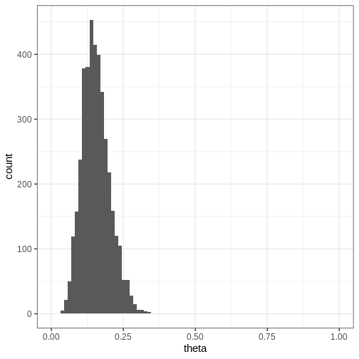
Compute the 95% credible intervals for the samples drawn with Stan. What is the probability that \(\theta \in (0.05, 0.15)\)? Plot a histogram of the posterior samples.
R
CI95 <- quantile(theta_samples, probs = c(0.025, 0.975))
theta_between_0.05_0.15 <- mean(theta_samples>0.05 & theta_samples<0.15)


p <- ggplot(data = data.frame(theta = theta_samples)) +
  geom_histogram(aes(x = theta), bins = 30) +
  coord_cartesian(xlim = c(0, 1))


print(p)
Challenge
Try modifying the Stan program so that you add a \(Beta(\alpha, \beta)\) prior for \(\theta\).
Can you modify the Stan program further so that you can set the hyperparameters \(\alpha, \beta\) as part of the data? What is the benefit of using this approach?
Modifying the data block so that it declares the hyperparameters as
data (e.g. real<lower=0> alpha;) enables setting the
hyperparameter values as part of data. This makes it possible to change
the hyperparameters without modifying the Stan file.
Additional Stan blocks
In addition to the data, parameters, and model blocks there are additional blocks that can be included in the program.
Functions: For user-defined functions. This block must be the first in the Stan program. It allows users to define custom functions.
Transformed data: This block is used for transformations of the data variables. It is often employed to preprocess or modify the input data before it is used in the main model. Common tasks include standardization, scaling, or other data adjustments.
Transformed parameters: In this block, transformations of the parameters are defined. If transformed parameters are used on the left-hand side of sampling statements in the model block, the Jacobian adjustment for the posterior density needs to be included in the model block as well.
Generated quantities: This block is used to define quantities based on both data and model parameters. These quantities are not part of the model but are useful for post-processing.
We will make use of these additional structures in subsequent illustrations.
Example 2: Normal model
Next, let’s implement the normal model in Stan. First we’ll generate some data \(X\) from a normal model with unknown mean and standard deviation parameters \(\mu\) and \(\sigma\)
R
# Sample size
N <- 99

# Generate data with unknown parameters
unknown_sigma <- runif(1, 0, 10)
unknown_mu <- runif(1, -5, 5)

X <- rnorm(n = N,
           mean = unknown_mu,
           sd = unknown_sigma)

normal_data <- list(N = N, X = X)
The Stan program for the normal model is specified in the next code chunk. It introduces a new data type (vector) and leverages vectorization in the likelihood statement. In the end of the program, a generated quantities block is included which generates new data (X_tilde) to estimate what unseen data points might look like. This resulting distribution is referred to as the posterior predictive distribution, which is generated by drawing a random realization from the normal distribution for each posterior sample \((\mu, \sigma)\).
STAN
data {
  int<lower=0> N;
  vector[N] X;
}
parameters {
  real mu;
  real<lower=0> sigma;
}
model {
  // Vectorized likelihood
  X ~ normal(mu, sigma);

  // Priors
  mu ~ normal(0, 1);
  sigma ~ gamma(2, 1);
}
generated quantities {
  real X_tilde;
  X_tilde = normal_rng(mu, sigma);
}
Let’s fit the model to the data
R
normal_samples <- rstan::sampling(normal_model,
                                  normal_data)
OUTPUT
SAMPLING FOR MODEL 'anon_model' NOW (CHAIN 1).
Chain 1:
Chain 1: Gradient evaluation took 5e-06 seconds
Chain 1: 1000 transitions using 10 leapfrog steps per transition would take 0.05 seconds.
Chain 1: Adjust your expectations accordingly!
Chain 1:
Chain 1:
Chain 1: Iteration: 1 / 2000 [ 0%] (Warmup)
Chain 1: Iteration: 200 / 2000 [ 10%] (Warmup)
Chain 1: Iteration: 400 / 2000 [ 20%] (Warmup)
Chain 1: Iteration: 600 / 2000 [ 30%] (Warmup)
Chain 1: Iteration: 800 / 2000 [ 40%] (Warmup)
Chain 1: Iteration: 1000 / 2000 [ 50%] (Warmup)
Chain 1: Iteration: 1001 / 2000 [ 50%] (Sampling)
Chain 1: Iteration: 1200 / 2000 [ 60%] (Sampling)
Chain 1: Iteration: 1400 / 2000 [ 70%] (Sampling)
Chain 1: Iteration: 1600 / 2000 [ 80%] (Sampling)
Chain 1: Iteration: 1800 / 2000 [ 90%] (Sampling)
Chain 1: Iteration: 2000 / 2000 [100%] (Sampling)
Chain 1:
Chain 1: Elapsed Time: 0.008 seconds (Warm-up)
Chain 1: 0.007 seconds (Sampling)
Chain 1: 0.015 seconds (Total)
Chain 1:
SAMPLING FOR MODEL 'anon_model' NOW (CHAIN 2).
Chain 2:
Chain 2: Gradient evaluation took 2e-06 seconds
Chain 2: 1000 transitions using 10 leapfrog steps per transition would take 0.02 seconds.
Chain 2: Adjust your expectations accordingly!
Chain 2:
Chain 2:
Chain 2: Iteration: 1 / 2000 [ 0%] (Warmup)
Chain 2: Iteration: 200 / 2000 [ 10%] (Warmup)
Chain 2: Iteration: 400 / 2000 [ 20%] (Warmup)
Chain 2: Iteration: 600 / 2000 [ 30%] (Warmup)
Chain 2: Iteration: 800 / 2000 [ 40%] (Warmup)
Chain 2: Iteration: 1000 / 2000 [ 50%] (Warmup)
Chain 2: Iteration: 1001 / 2000 [ 50%] (Sampling)
Chain 2: Iteration: 1200 / 2000 [ 60%] (Sampling)
Chain 2: Iteration: 1400 / 2000 [ 70%] (Sampling)
Chain 2: Iteration: 1600 / 2000 [ 80%] (Sampling)
Chain 2: Iteration: 1800 / 2000 [ 90%] (Sampling)
Chain 2: Iteration: 2000 / 2000 [100%] (Sampling)
Chain 2:
Chain 2: Elapsed Time: 0.009 seconds (Warm-up)
Chain 2: 0.008 seconds (Sampling)
Chain 2: 0.017 seconds (Total)
Chain 2:
SAMPLING FOR MODEL 'anon_model' NOW (CHAIN 3).
Chain 3:
Chain 3: Gradient evaluation took 4e-06 seconds
Chain 3: 1000 transitions using 10 leapfrog steps per transition would take 0.04 seconds.
Chain 3: Adjust your expectations accordingly!
Chain 3:
Chain 3:
Chain 3: Iteration: 1 / 2000 [ 0%] (Warmup)
Chain 3: Iteration: 200 / 2000 [ 10%] (Warmup)
Chain 3: Iteration: 400 / 2000 [ 20%] (Warmup)
Chain 3: Iteration: 600 / 2000 [ 30%] (Warmup)
Chain 3: Iteration: 800 / 2000 [ 40%] (Warmup)
Chain 3: Iteration: 1000 / 2000 [ 50%] (Warmup)
Chain 3: Iteration: 1001 / 2000 [ 50%] (Sampling)
Chain 3: Iteration: 1200 / 2000 [ 60%] (Sampling)
Chain 3: Iteration: 1400 / 2000 [ 70%] (Sampling)
Chain 3: Iteration: 1600 / 2000 [ 80%] (Sampling)
Chain 3: Iteration: 1800 / 2000 [ 90%] (Sampling)
Chain 3: Iteration: 2000 / 2000 [100%] (Sampling)
Chain 3:
Chain 3: Elapsed Time: 0.008 seconds (Warm-up)
Chain 3: 0.007 seconds (Sampling)
Chain 3: 0.015 seconds (Total)
Chain 3:
SAMPLING FOR MODEL 'anon_model' NOW (CHAIN 4).
Chain 4:
Chain 4: Gradient evaluation took 2e-06 seconds
Chain 4: 1000 transitions using 10 leapfrog steps per transition would take 0.02 seconds.
Chain 4: Adjust your expectations accordingly!
Chain 4:
Chain 4:
Chain 4: Iteration: 1 / 2000 [ 0%] (Warmup)
Chain 4: Iteration: 200 / 2000 [ 10%] (Warmup)
Chain 4: Iteration: 400 / 2000 [ 20%] (Warmup)
Chain 4: Iteration: 600 / 2000 [ 30%] (Warmup)
Chain 4: Iteration: 800 / 2000 [ 40%] (Warmup)
Chain 4: Iteration: 1000 / 2000 [ 50%] (Warmup)
Chain 4: Iteration: 1001 / 2000 [ 50%] (Sampling)
Chain 4: Iteration: 1200 / 2000 [ 60%] (Sampling)
Chain 4: Iteration: 1400 / 2000 [ 70%] (Sampling)
Chain 4: Iteration: 1600 / 2000 [ 80%] (Sampling)
Chain 4: Iteration: 1800 / 2000 [ 90%] (Sampling)
Chain 4: Iteration: 2000 / 2000 [100%] (Sampling)
Chain 4:
Chain 4: Elapsed Time: 0.008 seconds (Warm-up)
Chain 4: 0.008 seconds (Sampling)
Chain 4: 0.016 seconds (Total)
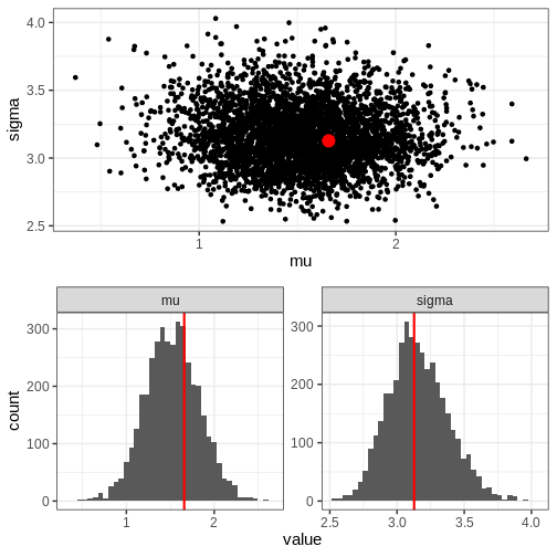
Chain 4: Next, we’ll extract posterior samples and generate a plot for the joint, and marginal posteriors. The true unknown parameter values are included in the plots in red.
R
# Extract parameter samples
par_samples <- rstan::extract(normal_samples, c("mu", "sigma")) %>%
  do.call(cbind, .) %>%
  data.frame


# Full posterior
p_posterior <- ggplot(data = par_samples) +
  geom_point(aes(x = mu, y = sigma)) +
  annotate("point", x = unknown_mu, y = unknown_sigma,
           color = "red", size = 5)

# Marginal posteriors
p_marginals <- ggplot(data = par_samples %>% gather) +
  geom_histogram(aes(x = value), bins = 40) +
  geom_vline(data = data.frame(key = c("mu", "sigma"),
                               value = c(unknown_mu, unknown_sigma)),
             aes(xintercept = value), color = "red", linewidth = 1) +
  facet_wrap(~key, scales = "free")


p <- cowplot::plot_grid(p_posterior, p_marginals,
                        ncol = 1)

print(p)
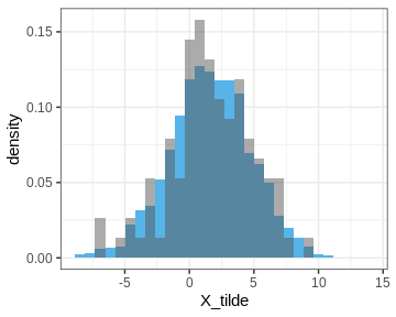
Let’s also plot the posterior predictive distribution samples histogram and compare it to that of the data.
R
PPD <- rstan::extract(normal_samples, c("X_tilde"))[[1]] %>%
  data.frame(X_tilde = . )

p_PPD <- ggplot() +
  geom_histogram(data = PPD,
                 aes(x = X_tilde, y = after_stat(density)),
                 bins = 30, fill = posterior_color) +
  geom_histogram(data = data.frame(X), aes(x = X, y = after_stat(density)),
                 bins = 30, alpha = 0.5)

print(p_PPD)
Example 3: Linear regression
Challenge
Write a Stan program for linear regression with one dependent variable.
Generate data from the linear model and use the Stan program to estimate the intercept \(\alpha\), slope \(\beta\), and noise term \(\sigma\).
STAN
data {
  int<lower=0> N; // Sample size
  vector[N] x; // x-values
  vector[N] y; // y-values
}
parameters {
  real alpha; // intercept
  real beta;  // slope
  real<lower=0> sigma; // noise
}

model {

  // Likelihood
  y ~ normal(alpha + beta * x, sigma);

  // Priors
  alpha ~ normal(0, 1);
  beta ~ normal(0, 1);
  sigma ~ inv_gamma(1, 1);
}
Challenge
Modify the program for linear regression so it facilitates \(M\) dependent variables.
STAN
data {
  int<lower=0> N; // Sample size
  int<lower=0> M; // Number of features
  matrix[N, M] x; // x-values
  vector[N] y; // y-values
}
parameters {
  real alpha; // intercept
  vector[M] beta;  // slopes
  real<lower=0> sigma; // noise
}

model {

  // Likelihood
  y ~ normal(alpha + x * beta, sigma);

  // Priors
  alpha ~ normal(0, 1);
  beta ~ normal(0, 1);
  sigma ~ inv_gamma(1, 1);
}- Stan is a tool for efficient posterior distribution sample generation.
- A Stan program is specified in a separate text file that consists of code blocks, with the data, parameters, and model blocks being the most crucial ones.
Resources
- Official release paper https://www.jstatsoft.org/article/view/v076i01
- User’s guide https://mc-stan.org/docs/2_18/stan-users-guide/
- Function’s reference https://mc-stan.org/docs/functions-reference/
- Reference manual https://mc-stan.org/docs/reference-manual/
- Stan forum https://discourse.mc-stan.org
- Case studies https://mc-stan.org/users/documentation/case-studies
Reading
- BDA3: Ch. 12.6, Appendix C
- Bayes Rules!: Ch. 6.2