Hierarchical models
Last updated on 2025-11-10 | Edit this page
Estimated time: 14 minutes
Overview
Questions
- How does Bayesian modeling accommodate group structure?
Objectives
- Learn to construct and fit hierarchical models.
Hierarchical (or multi-level) models are a class of models suited for situations where the study population comprises distinct but interconnected groups. For example, analyzing student performance across different schools, income disparities among various regions, or studying animal behavior within different populations are scenarios where such models would be appropriate.
Incorporating group-wise parameters allows us to model each group separately, and a model becomes hierarchical when we treat the parameters of the prior distribution as unknown. These parameters, known as hyperparameters, are assigned their own prior distribution, referred to as a hyperprior, and are learned during the model fitting process. Similarly as priors, the hyperpriors should be set so they reflect ranges of possible hyperparameter values. Conceptually, these hyperparameters and hyperpriors operate at a higher level of hierarchy, hence the name.
For example, let’s consider the beta-binomial model discussed in Episode 1. We used it to estimate the prevalence of left-handedness based on a sample of 50 students. If we were to include additional information, such as the students’ majors, we could extend the model as follows:
\[X_g \sim \text{Bin}(N_g, \theta_g) \\ \theta_g \sim \text{Beta}(\alpha, \beta) \\ \alpha, \beta \sim \Gamma(2, 0.1).\]
Here, the subscript \(g\) indexes the groups based on majors. The group-specific prevalences for left-handedness \(\theta_g\) are assigned a beta prior with hyperparameters \(\alpha\) and \(\beta\) which are treated as random variables. The final line indicates the hyperprior \(\Gamma(2, 0.1)\) governing the prior beliefs about the hyperparameters.
In this hierarchical beta-binomial model, students are considered exchangeable within their majors but no longer across the entire population. However, an underlying assumption of similarity exists between the groups since they share a common prior, that is learned. This way the groups are not entirely independent but are not treated as equal either.
One of the key advantages of Bayesian hierarchical models is their capacity to leverage information across groups. By pooling information from various groups, these models can yield more robust estimates, particularly when data availability is limited.
Another distinction from non-hierarchical models is that the prior, or the population distribution, of the parameters is learned in the process. This population distribution can provide information into parameter variability on a broader scale, even for groups where data is scarce or completely missing. For instance, if we had data on the handedness of students majoring in natural sciences, the population distribution can give insights into students in humanities and social sciences as well.
In the following example, we will perform a hierarchical analysis of human heights across different countries.
Example: human height
Let’s examine the heights of adults in various countries. In [1], averages and standard errors of adult heights in centimeters across different countries and age groups were provided. We’ll utilize this dataset to generate a sample of hypothetical individual heights and then assess our ability to reproduce these measured height statistics.
This approach is commonly employed when building and testing models: we generate simulated data with known parameters and then compare the inferred results to these known parameters. In our case, the true parameters are derived from real-world data.
We’ll employ a normal model with unknown mean \(\mu\) and standard deviation \(\sigma\) as our generative model, and treat these parameters hierarchically.
First, let’s load the data and examine its structure.
R
set.seed(4985)

height <- read.csv("data/height_data.csv")
str(height)
OUTPUT
'data.frame':	210000 obs. of  8 variables:
 $ Country                                   : chr  "Afghanistan" "Afghanistan" "Afghanistan" "Afghanistan" ...
 $ Sex                                       : chr  "Boys" "Boys" "Boys" "Boys" ...
 $ Year                                      : int  1985 1985 1985 1985 1985 1985 1985 1985 1985 1985 ...
 $ Age.group                                 : int  5 6 7 8 9 10 11 12 13 14 ...
 $ Mean.height                               : num  103 109 115 120 125 ...
 $ Mean.height.lower.95..uncertainty.interval: num  92.9 99.9 106.3 112.2 117.9 ...
 $ Mean.height.upper.95..uncertainty.interval: num  114 118 123 128 132 ...
 $ Mean.height.standard.error                : num  5.3 4.72 4.27 3.92 3.66 ...
Let’s subset this data to simplify the analysis and focus on the height of adult women measured in 2019.
R
height_women <- height %>%
  filter(
    Age.group == 19,
    Sex == "Girls",
    Year == 2019
    ) %>%
  # Select variables of interest
  select(Country, Sex, Mean.height, Mean.height.standard.error)
Let’s select 10 countries randomly
R
set.seed(5431)
# Select countries
N_countries <- 10
Countries <- sample(unique(height_women$Country),
                    size = N_countries,
                    replace = FALSE) %>% sort

height_women10 <- height_women %>% filter(Country %in% Countries)

height_women10
OUTPUT
         Country   Sex Mean.height Mean.height.standard.error
1     Bangladesh Girls    152.3776                  0.4966124
2         Belize Girls    158.1201                  1.4026324
3       Cameroon Girls    160.4112                  0.6146315
4           Chad Girls    162.1242                  0.8894219
5  Cote d'Ivoire Girls    158.6524                  0.9254438
6          Ghana Girls    158.8551                  0.8002225
7          Kenya Girls    159.4338                  0.6680202
8     Luxembourg Girls    165.0690                  1.3778094
9         Taiwan Girls    160.6953                  0.7307839
10     Venezuela Girls    160.0370                  1.0813162
Simulate data
Now, we can treat the values in the table above as ground truth and simulate some data based on them. Let’s generate \(N=10\) samples for each country from the normal model with \(\mu = \text{Mean.height}\) and \(\sigma = \text{Mean.height.standard.error}\).
R
# Sample size per group
N <- 10

# For each country, generate heights
height_sim <- lapply(1:N_countries, function(i) {

  my_df <- height_women10[i, ]

  data.frame(Country = my_df$Country,
             # Random values from normal
             Height = rnorm(N,
                            mean = my_df$Mean.height,
                            sd = my_df$Mean.height.standard.error))

}) %>%
  do.call(rbind, .)
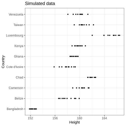
Let’s plot the data
R
# Plot
height_sim %>%
    ggplot() +
    geom_point(aes(x = Height, y = Country)) +
    labs(title = "Simulated data")
Modeling
Let’s build a normal model that uses partial pooling for the country means and standard deviations. The model can be stated as follows:
\[\begin{align} X_{gi} &\sim \text{N}(\mu_g, \sigma_g) \\ \mu_g &\sim \text{N}(\mu_\mu, \sigma_\mu) \\ \sigma_g &\sim \Gamma(\alpha_\sigma, \beta_\sigma) \\ \mu_\mu &\sim \text{N}(0, 100)\\ \sigma_\mu &\sim \Gamma(2, 0.1) \\ \alpha_\sigma, \beta_\sigma &\sim \Gamma(2, 0.01). \end{align}\]
Above, \(X_{gi}\) denotes the height for individual \(i\) in country \(g\). The country specific parameters \(\mu_g\) and \(\sigma_g\) are given normal and gamma priors, respectively, with unknown hyperparameters that, in turn, are given hyperpriors on the last two lines. The hyperpriors are quite uninformative as they allow large hyperparameter ranges.
Below is the Stan program for this model. The data points are input
as a concatenated vector X. The country-specific start and
end indices are computed in the transformed data block. This approach
accommodates uneven sample sizes between groups, although in our data
these are equal.
The parameters block contains the declarations of mean and standard deviation vectors, along with the hyperparameters. The hyperparameter subscripts denote the parameter they are assigned to so, for instance, \(\sigma_{\mu}\) is the standard deviation of the mean parameter \(\mu\). The generated quantities block generates samples from the population distributions of \(\mu\) and \(\sigma\) and a country-agnostic posterior predictive distribution \(\tilde{X}\).
STAN
data {
  int<lower=0> G; // number of groups
  int<lower=0> N[G]; // sample size within each group
  vector[sum(N)] X; // concatenated observations
}

transformed data {
  // get first and last index for each group in X
  int start_i[G];
  int end_i[G];

  for(g in 1:G) {

    if(g == 1) {
      start_i[1] = 1;
    } else {
      start_i[g] = start_i[g-1] + N[g-1];
    }

    end_i[g] = start_i[g] + N[g]-1;
  }
}

parameters {

  // parameters
  vector[G] mu;
  vector<lower=0>[G] sigma;

  // hyperparameters
  real mu_mu;
  real<lower=0> sigma_mu;
  real<lower=0> alpha_sigma;
  real<lower=0> beta_sigma;
}

model {

  // Likelihood for each group
  for(i in 1:G) {
    X[start_i[i]:end_i[i]] ~ normal(mu[i], sigma[i]);
  }

  // Priors
  mu ~ normal(mu_mu, sigma_mu);
  sigma ~ gamma(alpha_sigma, beta_sigma);

  // Hyperpriors
  mu_mu ~ normal(0, 100);
  sigma_mu ~ gamma(2, 0.1);
  alpha_sigma ~ gamma(2, 0.01);
  beta_sigma ~ gamma(2, 0.01);
}

generated quantities {

  real mu_tilde;
  real<lower=0> sigma_tilde;
  real X_tilde;

  // Population distributions
  mu_tilde = normal_rng(mu_mu, sigma_mu);
  sigma_tilde = gamma_rng(alpha_sigma, beta_sigma);

  // Posterior predictive distribution
  X_tilde = normal_rng(mu_tilde, sigma_tilde);

}
Now we can call Stan and fit the model. Hierarchical models can
encounter convergence issues and for this reason, we’ll use 10000
iterations and set adapt_delta = 0.99. This controls the
acceptance probability in Stan’s adaptation period and will result in a
smaller step size in the Markov chain. Moreover, we’ll speed up the
inference by running 2 chains in parallel by setting
cores = 2.
R
stan_data <- list(G = length(unique(height_sim$Country)),
                  N = rep(N, length(Countries)),
                  X = height_sim$Height)

normal_hier_fit <- rstan::sampling(normal_hier_model,
                                   stan_data,
                                   iter = 10000,
                                   chains = 2,
                                   # Use to avoid divergent transitions:
                                   control = list(adapt_delta = 0.99),
                                   cores = 2)
For comparison, we will also run an unpooled analysis of heights, which makes use of the following Stan file:
R
unpooled_summaries <- list()

for(i in 1:N_countries) {

  my_country <- unique(height_sim$Country)[i]

  my_df <- height_sim %>%
    filter(Country == my_country)

  my_stan_data <- list(N =  my_df %>% nrow,
                       X = my_df$Height)

  my_fit <- rstan::sampling(normal_pooled_model,
                              my_stan_data,
                              iter = 10000,
                              chains = 2,
                                    # Use to get rid of divergent transitions:
                                    control = list(adapt_delta = 0.99),
                              cores = 2,
                            refresh = 0
                            )


  unpooled_summaries[[i]] <- rstan::summary(my_fit, c("mu", "sigma"))$summary %>%
  data.frame() %>%
  rownames_to_column(var = "par") %>%
  mutate(country = my_country)

}


unpooled_summaries <- do.call(rbind, unpooled_summaries)
Country-specific estimates
Let’s first compare the marginal posteriors for the country-specific estimates from the hierarchical model (blue) and an unpooled model (brown) that treats the parameters separately.
R
par_summary <- rstan::summary(normal_hier_fit, c("mu", "sigma"))$summary %>%
  data.frame() %>%
  rownames_to_column(var = "par") %>%
  separate(par, into = c("par", "country"), sep = "\\[") %>%
  mutate(country = gsub("\\]", "", country)) %>%
  mutate(country = Countries[as.integer(country)])

ggplot() +
geom_errorbar(data = par_summary, aes(x = country, ymin = X2.5., ymax = X97.5.),
              color = posterior_color) +
geom_point(data = height_women10 %>%
             rename_with(~ c('mu', 'sigma'), 3:4) %>%
             gather(key = "par",
                    value = "value",
                    -c(Country, Sex)),
           aes(x = Country, y = value)) +
geom_errorbar(data = unpooled_summaries,
              aes(x = country, ymin = X2.5., ymax = X97.5.),
              color = "brown") +
facet_wrap(~ par, scales = "free", ncol = 1) +
coord_flip()
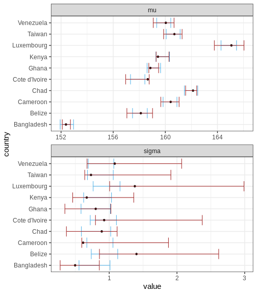
Above, the black points represent the true values, and the intervals are the 95% CIs for a hierarchical and non-hierarchical models, respectively. As apparent, the CIs from the hierarchical model are more concentrated and better capture the true values.
Challenge
Experiment with the data and fit. Explore the effect of sample size, unequal sample sizes between countries, and the amount of countries, for example.
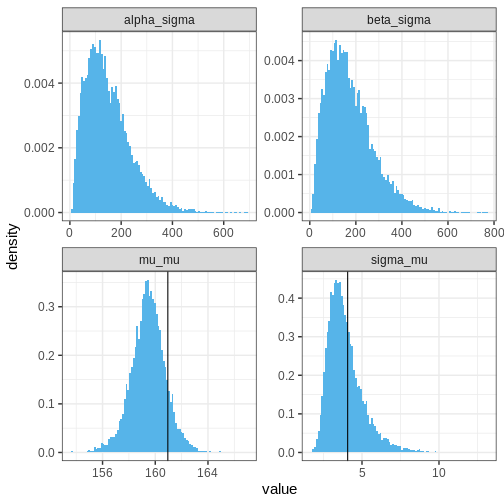
Hyperparameters
Let’s then plot the population distribution’s parameters, that is, the hyperparameters. The sample-based values are included in the plots of \(\mu_\mu\) and \(\sigma_\mu\) (why not for the other two hyperparameters?). It seems that the model has slightly underestimated the overall average and variance of the mean parameter \(\mu\), which is not suprising given the low number of data points.
R
## Population distributions:
population_samples_l <- rstan::extract(normal_hier_fit,
                                       c("mu_mu", "sigma_mu", "alpha_sigma", "beta_sigma")) %>%
  do.call(cbind, .) %>%
  set_colnames(c("mu_mu", "sigma_mu", "alpha_sigma", "beta_sigma")) %>%
  data.frame() %>%
  mutate(sample = 1:nrow(.)) %>%
  gather(key = "hyperpar", value = "value", -sample)


ggplot() +
  geom_histogram(data = population_samples_l,
                 aes(x = value, y = after_stat(density)),
                 fill = posterior_color,
                 bins = 100) +
  geom_vline(data = height_women %>%
               rename_with(~ c('mu', 'sigma'), 3:4) %>%
               filter(Sex == "Girls") %>%
               summarise(mu_mu = mean(mu), sigma_mu = sd(mu)) %>%
               gather(key = "hyperpar", value = "value"),
             aes(xintercept = value)
             )+
  facet_wrap(~hyperpar, scales = "free")
Population distributions
Let’s then plot the population distributions and compare to the true sample means and standard errors.
R
population_l <- rstan::extract(normal_hier_fit, c("mu_tilde", "sigma_tilde")) %>%
  do.call(cbind, .) %>%
  data.frame() %>%
  set_colnames( c("mu", "sigma")) %>%
  mutate(sample = 1:nrow(.)) %>%
  gather(key = "par", value = "value", -sample)


ggplot() +
  geom_histogram(data = population_l,
                 aes(x = value, y = after_stat(density)),
                 bins = 100, fill = posterior_color) +
    geom_histogram(data = height_women %>%
                     rename_with(~ c('mu', 'sigma'), 3:4) %>%
                     gather(key = "par", value = "value", -c(Country, Sex)) %>%
                     filter(Sex == "Girls"),
                   aes(x = value, y = after_stat(density)),
                   alpha = 0.75, bins = 30) +
  facet_wrap(~par, scales = "free") +
  labs(title = "Blue = posterior; black = sample")
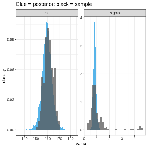 We can see that the population distribution is able to capture the
measured average heights and standard deviations relatively well,
although the within-country variation is estimated to be too
concentrated. However, remember that these estimates are based on a
limited sample: 10 out of 200 countries with 10 individuals in each
group.
We can see that the population distribution is able to capture the
measured average heights and standard deviations relatively well,
although the within-country variation is estimated to be too
concentrated. However, remember that these estimates are based on a
limited sample: 10 out of 200 countries with 10 individuals in each
group.
Posterior predictive distribution
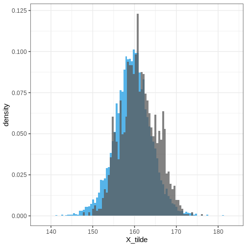
Finally, let’s plot the posterior predictive distribution for the whole population and overlay it with the simulated data based on all countries.
R
# For each country, generate some random girl's heights
height_all <- lapply(1:nrow(height_women), function(i) {

  my_df <- height_women[i, ] %>%
    rename_with(~ c('mu', 'sigma'), 3:4)

  data.frame(Country = my_df$Country,
             Sex = my_df$Sex,
             # Random normal values based on sample mu and sd
             Height = rnorm(N, my_df$mu, my_df$sigma))

}) %>%
  do.call(rbind, .)
R
# Extract the posterior predictive distribution
PPD <- rstan::extract(normal_hier_fit, c("X_tilde")) %>%
  data.frame() %>%
  set_colnames( c("X_tilde")) %>%
  mutate(sample = 1:nrow(.))


ggplot() +
  geom_histogram(data = PPD,
                 aes(x = X_tilde, y = after_stat(density)),
                 bins = 100,
                 fill = posterior_color) +
  geom_histogram(data = height_all,
                 aes(x = Height, y = after_stat(density)),
                 alpha = 0.75,
                 bins = 100)
Extensions
Here, we analyzed the height for women in a randomly chosen countries using a hierarchical model. The model could be extended further, for instance, by adding hierarchy between sexes, continents, developed/developing countries etc.
- Hierarchical models are appropriate for scenarios where the study population naturally divides into subgroups.
- Hierarchical models borrow statistical strength across the population groups.
- Population distributions hold information about the variation of the model parameters over the whole population.
Reading
- Bayesian Data Analysis (3rd ed.): Ch. 5
- Statistical Rethinking (2nd ed.): Ch. 13
- Bayes Rules!: Ch. 15-19
References
[1] Height: Height and body-mass index trajectories of school-aged children and adolescents from 1985 to 2019 in 200 countries and territories: a pooled analysis of 2181 population-based studies with 65 million participants. Lancet 2020, 396:1511-1524