Short introduction to Bayesian statistics
Last updated on 2025-11-10 | Edit this page
Estimated time: 68 minutes
Overview
Questions
- How are statistical models formulated and fitted within the Bayesian framework?
Objectives
Learn to
- formulate prior, likelihood, posterior distributions.
- fit a Bayesian model with the grid approximation.
- communicate posterior information.
- work with with posterior samples.
Bayes’ formula
The starting point of Bayesian statistics is Bayes’ theorem, expressed as:
\[ p(\theta | X) = \frac{p(X | \theta) p(\theta) }{p(X)} \\ \]
When dealing with a statistical model, this theorem is used to infer the probability distribution of the model parameters \(\theta\), conditional on the available data \(X\). These probabilities are quantified by the posterior distribution \(p(\theta | X)\), which is primary the target of probabilistic modeling.
On the right-hand side of the formula, the likelihood function \(p(X | \theta)\) gives plausibility of the data given \(\theta\), and determines the impact of the data on the posterior.
A defining feature of Bayesian modeling is the second term in the numerator, the prior distribution \(p(\theta)\). The prior is used to incorporate beliefs about \(\theta\) before considering the data.
The denominator on the right-hand side \(p(X)\) is called the marginal probability, and is often practically impossible to compute. For this reason the proportional version of Bayes’ formula is typically employed:
\[ p(\theta | X) \propto p(\theta) p(X | \theta). \]
The proportional Bayes’ formula yields an unnormalized posterior distribution, which can subsequently be normalized to obtain the posterior.
Example 1: handedness
Let’s illustrate the use of the Bayes’ theorem with an example.
Assume we are trying to estimate the prevalence of left-handedness in humans, based on a sample of \(N=50\) students, out of which \(x=7\) are left-handed and 43 right-handed.
The outcome is binary and the students are assumed to be independent (e.g. no twins), so the binomial distribution is the appropriate choice for likelihood:
\[ p(X|\theta) = Bin(7 | 50, \theta). \]
Without further justification, we’ll choose \(p(\theta) = Beta(\theta |1, 10)\) as the prior distribution, so the unnormalized posterior distribution is
\[ p(\theta | X) = \text{Bin}(7 | 50, \theta) \cdot \text{Beta}(\theta | 1, 10). \]
Below, we’ll plot these functions. Likelihood (which is not a distribution!) has been normalized for better illustration.
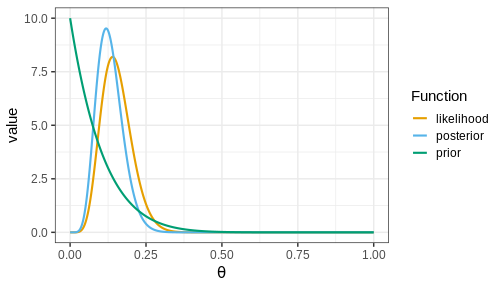
The figure shows that the majority of the mass in the posterior distribution is concentrated between 0 and 0.25. This implies that, given the available data and prior distribution, the model is fairly confident that the value of \(\theta\) is between these values. The peak of the posterior is at approximately 0.1 representing the most likely value. This aligns well with intuitive expectations about left-handedness in humans.
Actual value from a study from 1975 with 7,688 children in US grades 1-6 was 9.6%
Hardyck, C. et al. (1976), Left-handedness and cognitive deficit https://en.wikipedia.org/wiki/Handedness
Communicating posterior information
The posterior distribution \(p(\theta | X)\) contains all the information about \(\theta\) given the data, chosen model, and the prior distribution. However, understanding a distribution in itself can be challenging, especially if it is multidimensional. To effectively communicate posterior information, methods to quantify the information contained in the posterior are needed. Two commonly used types of estimates are point estimates, such as the posterior mean, mode, and variance, and posterior intervals, which provide probabilities for ranges of values.
Two specific types of posterior intervals are often of interest:
Credible intervals (CIs): These intervals leave equal posterior mass below and above them, computed as posterior quantiles. For instance, a 90% CI would span the range between the 5% and 95% quantiles.
Defined boundary intervals: Computed as the posterior mass for specific parts of the parameter space, these intervals quantify the probability for given parameter conditions. For example, we might be interested in the posterior probability that \(\theta > 0\), \(0<\theta<0.5\), or \(\theta<0\) or \(\theta > 0.5\). These probabilities can be computed by integrating the posterior over the corresponding sets.
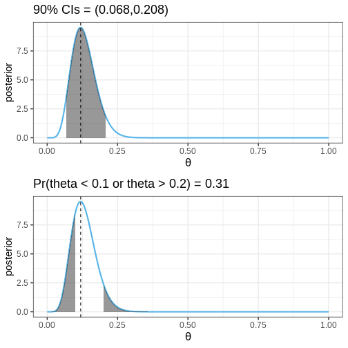
The following figures illustrate selected posterior intervals for the previous example along with the posterior mode, or maximum a posteriori (MAP) estimate.
Grid approximation
Specifying a probabilistic model can be simple, but a common bottleneck in Bayesian data analysis is model fitting. Later in the course, we will begin using Stan, a state-of-the-art method for approximating the posterior. However, we’ll begin fitting probabilistic model using the grid approximation. This approach involves computing the unnormalized posterior distribution at a grid of evenly spaced values in the parameter space and can be specified as follows:
- Define a grid of parameter values.
- Compute the prior and likelihood on the grid.
- Multiply to get the unnormalized posterior.
- Normalize.
Now, we’ll implement the grid approximation for the handedness example in R.
Example 2: handedness with grid approximation
First, we’ll load the required packages, define the data variables, and the grid of parameter values
R
# Sample size
N <- 50

# 7/50 are left-handed
x <- 7

# Define a grid of points in the interval [0, 1], with 0.01 interval
delta <- 0.01
theta_grid <- seq(from = 0, to = 1, by = delta)
Computing the values of the likelihood, prior, and unnormalized posterior is straightforward. While you can compute these using for-loops, vectorization as used below, is a more efficient approach:
R
likelihood <- dbinom(x = x, size = N, prob = theta_grid)
prior <- dbeta(theta_grid, 1, 10)
posterior <- likelihood*prior
Next, the posterior needs to be normalized.
In practice, this means dividing the values by the area under the unnormalized posterior. The area is computed with the integral \[\int_0^1 p(\theta | X)_{\text{unnormalized}} d\theta,\] which is for a grid approximated function is the sum \[\sum_{\text{grid}} p(\theta | X)_{\text{unnormalized}} \cdot \delta,\] where \(\delta\) is the grid interval.
R
# Normalize
posterior <- posterior/(sum(posterior)*delta)
# Likelihood also normalized for better visualization
likelihood <- likelihood/(sum(likelihood)*delta)
Finally, we can plot these functions
R
# Make data frame
df1 <- data.frame(theta = theta_grid, likelihood, prior, posterior)

# Wide to long format
df1_l <- df1 %>%
  gather(key = "Function", value = "value", -theta)

# Plot
p1 <- ggplot(df1_l,
       aes(x = theta, y = value, color = Function)) +
  geom_point(size = 2) +
  geom_line(linewidth = 1) +
  scale_color_grafify() +
  labs(x = expression(theta))

p1
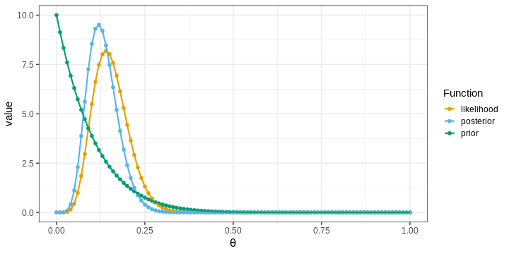
The points in the figure represent the values of the functions computed at the grid locations. The lines depict linear interpolations between these points.
Challenge
Experiment with different priors and examine their effects on the posterior. You could try, for example, different Beta distributions, the normal distribution, or the uniform distribution.
How does the shape of the prior impact the posterior?
What is the relationship between the posterior, data (likelihood) and the prior?
Grid approximation and posterior summaries
Next, we’ll learn how to compute point estimates and posterior intervals based on the approximate posterior obtained with the grid approximation.
Computing the posterior mean and variance is based on the definition of these statistics for continuous variables. The mean is defined as \[\int \theta \cdot p(\theta | X) d\theta,\] and can be computed using discrete integration: \[\sum_{\text{grid}} \theta \cdot p(\theta | X) \cdot \delta.\] Similarly, variance can be computed based on the definition \[\text{var}(\theta) = \int (\theta - \text{mean}(\theta))^2p(\theta | X)d\theta.\] Posterior mode is simply the grid value where the posterior is maximized.
In R, these statistics can be computed as follows:
R
data.frame(Estimate = c("Mode", "Mean", "Variance"),
           Value = c(df1[which.max(df1$posterior), "theta"],
                     sum(df1$theta*df1$posterior*delta),
                     sum(df1$theta^2*df1$posterior*delta) -
                       sum(df1$theta*df1$posterior*delta)^2))
OUTPUT
  Estimate       Value
1     Mode 0.120000000
2     Mean 0.131147540
3 Variance 0.001837869
Posterior intervals are also relatively easy to compute.
Finding the quantiles used to determine CIs is based on the cumulative distribution function of the posterior \(F(\theta) = \int_{\infty}^{\theta}p(y | X) dy\). The locations where the \(F(\theta) = 0.05\) and \(F(\theta) = 0.95\) define the 90% CIs.
Probabilities for certain parameter ranges are computed simply by integrating over the appropriate set, for example, \(Pr(\theta < 0.1) = \int_0^{0.1} p(\theta | X) d\theta.\)
Challenge
Compute the 90% CIs and the probability \(Pr(\theta < 0.1)\) for the handedness example.
R
# Quantiles
q5 <- theta_grid[which.max(cumsum(posterior)*delta > 0.05)]
q95 <- theta_grid[which.min(cumsum(posterior)*delta < 0.95)]

# Pr(theta < 0.1)
Pr_theta_under_0.1 <- sum(posterior[theta_grid < 0.1])*delta

print(paste0("90% CI = (", q5,",", q95,")"))
OUTPUT
[1] "90% CI = (0.07,0.21)"R
print(paste0("Pr(theta < 0.1) = ",
             round(Pr_theta_under_0.1, 5)))
OUTPUT
[1] "Pr(theta < 0.1) = 0.20659"Example 3: Gamma model with grid approximation
Let’s investigate another model and implement a grid approximation to fit it.
The gamma distribution arises, for example, in applications that model the waiting time between consecutive events. Let’s model the following data points as independent realizations from a \(\Gamma(\alpha, \beta)\) distribution with unknown shape \(\alpha\) and rate \(\beta\) parameters:
R
X <- c(0.34, 0.2, 0.22, 0.77, 0.46, 0.73, 0.24, 0.66, 0.64)
We’ll estimate \(\alpha\) and \(\beta\) using the grid approximation. Similarly as before, we’ll first need to define a grid. Since there are two parameters the parameter space is 2-dimensional and the grid needs to be defined at all pairwise combinations of the points of the individual grids.
R
delta <- 0.1
alpha_grid <- seq(from = 0.01, to = 15, by = delta)
beta_grid <- seq(from = 0.01, to = 25, by = delta)

# Get pairwise combinations
df2 <- expand.grid(alpha = alpha_grid, beta = beta_grid)
Next, we’ll compute the likelihood. As we assumed the data points to be independently generated from the gamma distribution, the likelihood is the product of the likelihoods of individual observations.
R
# Loop over all alpha, beta combinations
for(i in 1:nrow(df2)) {
  df2[i, "likelihood"] <- prod(
    dgamma(x = X,
           shape = df2[i, "alpha"],
           rate = df2[i, "beta"])
    )
}
Next, we’ll define priors for \(\alpha\) and \(\beta\). Only positive values are allowed, which should be reflected in the prior. We’ll use \(\Gamma\) priors with large variances.
Notice, that normalizing the posterior now requires integrating over both dimensions, hence the \(\delta^2\) below.
R
# Priors: alpha, beta ~ Gamma(2, .1)
df2 <- df2 %>%
  mutate(prior = dgamma(x = alpha, 2, 0.1)*dgamma(x = beta, 2, 0.1))

# Posterior
df2 <- df2 %>%
  mutate(posterior = prior*likelihood) %>%
  mutate(posterior = posterior/(sum(posterior)*delta^2)) # Normalize


# Plot
p_joint_posterior <- df2 %>%
  ggplot() +
  geom_tile(aes(x = alpha, y = beta, fill = posterior)) +
  scale_fill_gradientn(colours = rainbow(5)) +
  labs(x = expression(alpha), y = expression(beta))

p_joint_posterior
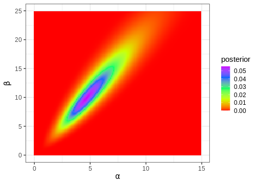
Next, we’ll compute the posterior mode, which is a point in the 2-dimensional parameter space.
R
df2[which.max(df2$posterior), c("alpha", "beta")]
OUTPUT
      alpha beta
14898  4.71 9.91
Often, in addition to the parameters of interest, the model contains parameters we are not interested in. For instance, we might only be interested in \(\alpha\), in which case \(\beta\) would be a ‘nuisance’ parameter. Nuisance parameters are part of the full (‘joint’) posterior, but they can be discarded by integrating the joint posterior over these parameters. A posterior integrated over some parameters is called a marginal posterior.
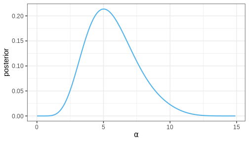
Let’s now compute the marginal posterior for \(\alpha\) by integrating over \(\beta\). Intuitively, it can be helpful to think of marginalization as a process where all of the joint posterior mass is drawn towards the \(\alpha\) axis, as if drawn by a gravitational force.
R
# Get marginal posterior for alpha
alpha_posterior <- df2 %>%
  group_by(alpha) %>%
  summarize(posterior = sum(posterior)) %>%
  mutate(posterior = posterior/(sum(posterior)*delta))

p_alpha_posterior <- alpha_posterior %>%
  ggplot() +
  geom_line(aes(x = alpha, y = posterior),
            color = posterior_color,
            linewidth = 1) +
  labs(x = expression(alpha))

p_alpha_posterior
Challenge
Does the MAP of the joint posterior of \(\theta = (\alpha, \beta)\) correspond to the MAPs of the marginal posteriors of \(\alpha\) and \(\beta\)?
The conjugate prior for the Gamma likelihood exists, which means there is a prior that causes the posterior to be of the same shape.
Working with samples
The main limitation of the grid approximation is that it becomes impractical for models with even a moderate number of parameters. The reason is that the number of computations grows as \(O \{ \Delta^p \}\) where \(\Delta\) is the number of grid points per model parameter and \(p\) the number of parameters. This quickly becomes prohibitive, and the grid approximation is seldom used in practice. The standard approach to fitting Bayesian models is to draw samples from the posterior with Markov chain Monte Carlo (MCMC) methods. These methods are the topic of a later episode but we’ll anticipate this now by studying how posterior summaries can be computed based on samples.
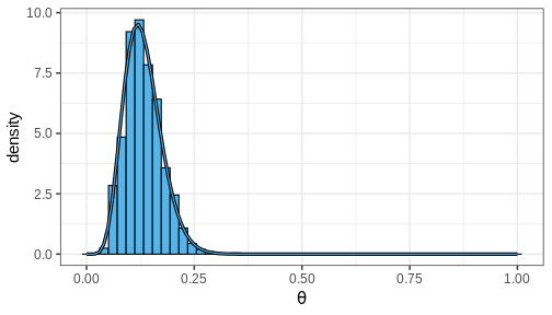
Example 4: handedness with samples
Let’s take the beta-binomial model (beta prior, binomial likelihood) of the handedness analysis as our example. It is an instance of a model for which the posterior can be computed analytically. Given a prior \(\text{Beta}(\alpha, \beta)\) and likelihood \(\text{Bin}(x | N, \theta)\), the posterior is \[p(\theta | X) = \text{Beta}(\alpha + x, \beta + N - x).\] Let’s generate \(n = 1000\) samples from this posterior using the handedness data:
R
n <- 1000
theta_samples <- rbeta(n, 1 + 7, 10 + 50 - 7)
Plotting a histogram of these samples against the grid approximation posterior displays that both are indeed approximating the same distribution
R
ggplot() +
  geom_histogram(data = theta_samples %>%
  data.frame(theta = .),
  aes(x = theta, y = after_stat(density)), bins = 50,
  fill = posterior_color, color = "black") +
    geom_line(data = df1,
            aes(x = theta, y = posterior),
            linewidth = 1.5) +
  geom_line(data = df1,
            aes(x = theta, y = posterior),
            color = posterior_color) +
  labs(x = expression(theta))
Computing posterior summaries from samples is easy. The posterior mean and variance are computed simply by taking the mean and variance of the samples, respectively. Posterior intervals are equally easy to compute: 90% CI is recovered from the appropriate quantiles and the probability of a certain parameter interval is the proportion of total samples within the interval.
Challenge
Compute the posterior mean, variance, 90% CI and \(Pr(\theta > 0.1)\) using the generated samples.
Posterior predictive distribution
Now we have learned how to fit a probabilistic model using the grid approximation and how to compute posterior summaries of the model parameters based on the fit or with posterior samples. A potentially interesting question that the posterior doesn’t directly answer is what do possible unobserved data values \(\tilde{X}\) look like, conditional on the observed values \(X\).
The unknown value can be predicted using the posterior predictive distribution \(p(\tilde{X} | X) = \int p(\tilde{X} | \theta) p(\theta | X) d\theta\). Using samples, this distribution can be sampled from by first drawing a value \(\theta^s\) from the posterior and then generating a random value from the likelihood function \(p(\tilde{X} | \theta^s)\).
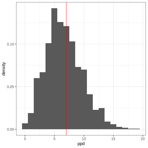
A posterior predictive distribution for the beta-binomial model, using the posterior samples of the previous example can be generated as
R
ppd <- rbinom(length(theta_samples), 50, prob = theta_samples)
In other words, this is the distribution of the number of left-handed people in a yet unseen sample of 50 people. Let’s plot the histogram of these samples and compare it to the observed data (red vertical line):
R
ggplot() +
  geom_histogram(data = data.frame(ppd),
                 aes(x = ppd, y = after_stat(density)), binwidth = 1) +
  geom_vline(xintercept = 7, color = "red")
- Likelihood determines the probability of data conditional on the model parameters.
- Prior encodes beliefs about the model parameters without considering data.
- Posterior quantifies the probability of parameter values conditional on the data.
- The posterior is a compromise between the data and prior. The less data available, the greater the impact of the prior.
- The grid approximation is a method for inferring the (approximate) posterior distribution.
- Posterior information can be summarized with point estimates and posterior intervals.
- The marginal posterior is accessed by integrating over nuisance parameters.
- Usually, Bayesian models are fitted using methods that generate samples from the posterior.
Reading
- Bayesian Data Analysis (3rd ed.): Ch. 1-3
- Statistical Rethinking (2nd ed.): Ch. 1-3
- Bayes Rules!: Ch. 1-6