Reshaping data with tidyr
Last updated on 2026-05-26 | Edit this page
Estimated time: 66 minutes
Overview
Questions
- How can I make my data into a longer format?
- How can I get my data into a wider format?
Objectives
- Use
pivot_longer()to reshape data into a longer format - Use
pivot_wider()to reshape data into a wider format
Motivation
Data come in a myriad of different shapes, and talking about data set can often become confusing as people are used to data being in different formats, and they call these formats different things. In the tidyverse, “tidy” data is a very opinionated term so that we can all talk about data with more common ground.
The goal of the tidyr package is to help you create tidy data.
Tidy data is data where:
- Every column is variable.
- Every row is an observation.
- Every cell is a single value.
Tidy data describes a standard way of storing data that is used
wherever possible throughout the tidyverse. If you ensure that your data
is tidy, you’ll spend less time fighting with the tools and more time
working on your analysis. Learn more about tidy data in
vignette("tidy-data").
Tall/long vs. wide data
Tall (or long) data are considered “tidy”, in that they adhere to the three tidy-data principles
Wide data are not necessarily “messy”, but have a shape less ideal for easy handling in the tidyverse
Example in longitudinal data design:
- wide data: each participant has a single row of data, with all
longitudinal observations in separate columns
- tall data: a participant has as many rows as longitudinal time points, with measures in separate columns
Creating longer data
Let us first talk about creating longer data. In most cases, you will encounter data that is in wide format, this is what is often taught in many disciplines and also necessary to run certain analyses in statistical programs like SPSS. In R, and specifically the tidyverse, working on long data has clear advantages, which we wil be exploring here while we also do the transformations.
As before, we need to start off by making sure we have the tidyverse package loaded, and the penguins dataset ready at hand.
In tidyverse, there is a single function to create longer data sets,
called pivot_longer. Those of you who might have some prior
experience with tidyverse, or you might encounter it when googling for
help, might have seen the gather function. This is an older
function of similar capabilities which we will not cover here, as the
pivot_longer function supersedes it.
R
penguins |>
  pivot_longer(contains("_"))
OUTPUT
# A tibble: 1,376 × 6
   species island    sex     year name               value
   <fct>   <fct>     <fct>  <int> <chr>              <dbl>
 1 Adelie  Torgersen male    2007 bill_length_mm      39.1
 2 Adelie  Torgersen male    2007 bill_depth_mm       18.7
 3 Adelie  Torgersen male    2007 flipper_length_mm  181
 4 Adelie  Torgersen male    2007 body_mass_g       3750
 5 Adelie  Torgersen female  2007 bill_length_mm      39.5
 6 Adelie  Torgersen female  2007 bill_depth_mm       17.4
 7 Adelie  Torgersen female  2007 flipper_length_mm  186
 8 Adelie  Torgersen female  2007 body_mass_g       3800
 9 Adelie  Torgersen female  2007 bill_length_mm      40.3
10 Adelie  Torgersen female  2007 bill_depth_mm       18
# ℹ 1,366 more rows
pivot_longer takes tidy-select column arguments, so it is easy to
grab all the columns you are after. Here, we are pivoting longer all
columns that contain an underscore. And what happens? We now have less
columns, but also two new columns we did not have before! In the
name column, all our previous columns names are, one after
the other. And in the value column, all the cell values for
the observations! So before, the data was wider, in that each of the
columns with _ had their own column, while now, they are
all collected into two columns instead of 4.
Why would we want to do that? Well, perhaps we want to plot all the
variables in a single ggplot call? Now that the measurement types are
collected in these two ways, we can facet over the name
column to create a sub-plot per measurement type!
R
penguins |>
  pivot_longer(contains("_")) |>
  ggplot(aes(y = value,
             x = species,
             fill = species)) +
  geom_boxplot() +
  facet_wrap(~name, scales = "free_y")
WARNING
Warning: Removed 8 rows containing non-finite outside the scale range
(`stat_boxplot()`).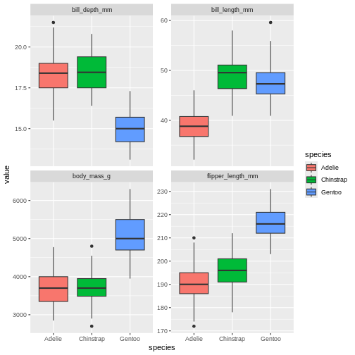
That’s pretty neat. By pivoting the data into this longer shape we are able to create sub-plots for all measurements easily with the same ggplot call and have them consistent, and nicely aligned. This longer format is also great for summaries, which we will be covering tomorrow.
Challenge 1
Pivot longer all columns ending with “mm” .
R
penguins |>
  pivot_longer(ends_with("mm"))
OUTPUT
# A tibble: 1,032 × 7
   species island    body_mass_g sex     year name              value
   <fct>   <fct>           <int> <fct>  <int> <chr>             <dbl>
 1 Adelie  Torgersen        3750 male    2007 bill_length_mm     39.1
 2 Adelie  Torgersen        3750 male    2007 bill_depth_mm      18.7
 3 Adelie  Torgersen        3750 male    2007 flipper_length_mm 181
 4 Adelie  Torgersen        3800 female  2007 bill_length_mm     39.5
 5 Adelie  Torgersen        3800 female  2007 bill_depth_mm      17.4
 6 Adelie  Torgersen        3800 female  2007 flipper_length_mm 186
 7 Adelie  Torgersen        3250 female  2007 bill_length_mm     40.3
 8 Adelie  Torgersen        3250 female  2007 bill_depth_mm      18
 9 Adelie  Torgersen        3250 female  2007 flipper_length_mm 195
10 Adelie  Torgersen          NA <NA>    2007 bill_length_mm     NA
# ℹ 1,022 more rows
Challenge 2
Pivot the penguins data so that all the bill measurements are in the same column.
R
penguins |>
  pivot_longer(starts_with("bill"))
OUTPUT
# A tibble: 688 × 8
   species island    flipper_length_mm body_mass_g sex     year name       value
   <fct>   <fct>                 <int>       <int> <fct>  <int> <chr>      <dbl>
 1 Adelie  Torgersen               181        3750 male    2007 bill_leng…  39.1
 2 Adelie  Torgersen               181        3750 male    2007 bill_dept…  18.7
 3 Adelie  Torgersen               186        3800 female  2007 bill_leng…  39.5
 4 Adelie  Torgersen               186        3800 female  2007 bill_dept…  17.4
 5 Adelie  Torgersen               195        3250 female  2007 bill_leng…  40.3
 6 Adelie  Torgersen               195        3250 female  2007 bill_dept…  18
 7 Adelie  Torgersen                NA          NA <NA>    2007 bill_leng…  NA
 8 Adelie  Torgersen                NA          NA <NA>    2007 bill_dept…  NA
 9 Adelie  Torgersen               193        3450 female  2007 bill_leng…  36.7
10 Adelie  Torgersen               193        3450 female  2007 bill_dept…  19.3
# ℹ 678 more rows
Challenge 3
As mentioned, pivot_longer accepts tidy-selectors. Pivot longer all numerical columns.
R
penguins |>
  pivot_longer(where(is.numeric))
OUTPUT
# A tibble: 1,720 × 5
   species island    sex    name               value
   <fct>   <fct>     <fct>  <chr>              <dbl>
 1 Adelie  Torgersen male   bill_length_mm      39.1
 2 Adelie  Torgersen male   bill_depth_mm       18.7
 3 Adelie  Torgersen male   flipper_length_mm  181
 4 Adelie  Torgersen male   body_mass_g       3750
 5 Adelie  Torgersen male   year              2007
 6 Adelie  Torgersen female bill_length_mm      39.5
 7 Adelie  Torgersen female bill_depth_mm       17.4
 8 Adelie  Torgersen female flipper_length_mm  186
 9 Adelie  Torgersen female body_mass_g       3800
10 Adelie  Torgersen female year              2007
# ℹ 1,710 more rows
Altering names during pivots
While often you can get away with leaving the default naming of the two columns as is, especially if you are just doing something quick like making a plot, most times you will likely want to control the names of your two new columns.
R
penguins |>
  pivot_longer(contains("_"),
               names_to = "columns",
               values_to = "content")
OUTPUT
# A tibble: 1,376 × 6
   species island    sex     year columns           content
   <fct>   <fct>     <fct>  <int> <chr>               <dbl>
 1 Adelie  Torgersen male    2007 bill_length_mm       39.1
 2 Adelie  Torgersen male    2007 bill_depth_mm        18.7
 3 Adelie  Torgersen male    2007 flipper_length_mm   181
 4 Adelie  Torgersen male    2007 body_mass_g        3750
 5 Adelie  Torgersen female  2007 bill_length_mm       39.5
 6 Adelie  Torgersen female  2007 bill_depth_mm        17.4
 7 Adelie  Torgersen female  2007 flipper_length_mm   186
 8 Adelie  Torgersen female  2007 body_mass_g        3800
 9 Adelie  Torgersen female  2007 bill_length_mm       40.3
10 Adelie  Torgersen female  2007 bill_depth_mm        18
# ℹ 1,366 more rows
Here, we change the “names” to “columns” and “values” to “content”. The pivot defaults are usually quite sensible, making it clear what is the column names and what are the cell values. But English might not be your working language or you might find something more obvious for your self.
But we have even more power in the renaming of columns. Pivots actually have quite a lot of options, making it possible for us to create outputs looking just like we want. Notice how the names of the columns we pivoted follow a specific structure. First is the name of the body part, then the type of measurement, then the unit of the measurement. This clear logic we can use to our advantage.
R
penguins |>
  pivot_longer(contains("_"),
               names_to = c("part", "measure" , "unit"),
               names_sep = "_")
OUTPUT
# A tibble: 1,376 × 8
   species island    sex     year part    measure unit   value
   <fct>   <fct>     <fct>  <int> <chr>   <chr>   <chr>  <dbl>
 1 Adelie  Torgersen male    2007 bill    length  mm      39.1
 2 Adelie  Torgersen male    2007 bill    depth   mm      18.7
 3 Adelie  Torgersen male    2007 flipper length  mm     181
 4 Adelie  Torgersen male    2007 body    mass    g     3750
 5 Adelie  Torgersen female  2007 bill    length  mm      39.5
 6 Adelie  Torgersen female  2007 bill    depth   mm      17.4
 7 Adelie  Torgersen female  2007 flipper length  mm     186
 8 Adelie  Torgersen female  2007 body    mass    g     3800
 9 Adelie  Torgersen female  2007 bill    length  mm      40.3
10 Adelie  Torgersen female  2007 bill    depth   mm      18
# ℹ 1,366 more rows
now, the pivot gave us 4 columns in stead of two! We told pivot that the column name could be split into the columns “part”, “measure” and “unit”, and that these were separated by underscore. Again we see how great consistent and logical naming of columns can be such a great help when working with data!
Challenge 4
Pivot longer all the bill measurements, and alter the names in one go, so that there are three columns named “part”, “measure” and “unit” after the pivot.
R
penguins |>
    pivot_longer(starts_with("bill"),
               names_to = c("part", "measure" , "unit"),
               names_sep = "_")
OUTPUT
# A tibble: 688 × 10
   species island  flipper_length_mm body_mass_g sex    year part  measure unit
   <fct>   <fct>               <int>       <int> <fct> <int> <chr> <chr>   <chr>
 1 Adelie  Torger…               181        3750 male   2007 bill  length  mm
 2 Adelie  Torger…               181        3750 male   2007 bill  depth   mm
 3 Adelie  Torger…               186        3800 fema…  2007 bill  length  mm
 4 Adelie  Torger…               186        3800 fema…  2007 bill  depth   mm
 5 Adelie  Torger…               195        3250 fema…  2007 bill  length  mm
 6 Adelie  Torger…               195        3250 fema…  2007 bill  depth   mm
 7 Adelie  Torger…                NA          NA <NA>   2007 bill  length  mm
 8 Adelie  Torger…                NA          NA <NA>   2007 bill  depth   mm
 9 Adelie  Torger…               193        3450 fema…  2007 bill  length  mm
10 Adelie  Torger…               193        3450 fema…  2007 bill  depth   mm
# ℹ 678 more rows
# ℹ 1 more variable: value <dbl>
Challenge 5
Pivot longer all the bill measurements, and use the
names_prefix argument. Give it the string “bill_”. What did
that do?
R
penguins |>
    pivot_longer(starts_with("bill"),
               names_prefix = "bill_")
OUTPUT
# A tibble: 688 × 8
   species island    flipper_length_mm body_mass_g sex     year name      value
   <fct>   <fct>                 <int>       <int> <fct>  <int> <chr>     <dbl>
 1 Adelie  Torgersen               181        3750 male    2007 length_mm  39.1
 2 Adelie  Torgersen               181        3750 male    2007 depth_mm   18.7
 3 Adelie  Torgersen               186        3800 female  2007 length_mm  39.5
 4 Adelie  Torgersen               186        3800 female  2007 depth_mm   17.4
 5 Adelie  Torgersen               195        3250 female  2007 length_mm  40.3
 6 Adelie  Torgersen               195        3250 female  2007 depth_mm   18
 7 Adelie  Torgersen                NA          NA <NA>    2007 length_mm  NA
 8 Adelie  Torgersen                NA          NA <NA>    2007 depth_mm   NA
 9 Adelie  Torgersen               193        3450 female  2007 length_mm  36.7
10 Adelie  Torgersen               193        3450 female  2007 depth_mm   19.3
# ℹ 678 more rows
Challenge 6
Pivot longer all the bill measurements, and use the
names_prefix, names_to and
names_sep arguments. What do you need to change in
names_to from the previous example to make it work now that
we also use names_prefix?
R
penguins |>
    pivot_longer(starts_with("bill"),
              names_prefix = "bill_",
              names_to = c("bill_measure" , "unit"),
              names_sep = "_")
OUTPUT
# A tibble: 688 × 9
   species island   flipper_length_mm body_mass_g sex    year bill_measure unit
   <fct>   <fct>                <int>       <int> <fct> <int> <chr>        <chr>
 1 Adelie  Torgers…               181        3750 male   2007 length       mm
 2 Adelie  Torgers…               181        3750 male   2007 depth        mm
 3 Adelie  Torgers…               186        3800 fema…  2007 length       mm
 4 Adelie  Torgers…               186        3800 fema…  2007 depth        mm
 5 Adelie  Torgers…               195        3250 fema…  2007 length       mm
 6 Adelie  Torgers…               195        3250 fema…  2007 depth        mm
 7 Adelie  Torgers…                NA          NA <NA>   2007 length       mm
 8 Adelie  Torgers…                NA          NA <NA>   2007 depth        mm
 9 Adelie  Torgers…               193        3450 fema…  2007 length       mm
10 Adelie  Torgers…               193        3450 fema…  2007 depth        mm
# ℹ 678 more rows
# ℹ 1 more variable: value <dbl>
Cleaning up values during pivots.
When pivoting, it is common that quite some NA values
appear in the values column. We can remove these immediately by making
the argument values_drop_na be TRUE
R
penguins |>
  pivot_longer(starts_with("bill"),
               values_drop_na = TRUE)
OUTPUT
# A tibble: 684 × 8
   species island    flipper_length_mm body_mass_g sex     year name       value
   <fct>   <fct>                 <int>       <int> <fct>  <int> <chr>      <dbl>
 1 Adelie  Torgersen               181        3750 male    2007 bill_leng…  39.1
 2 Adelie  Torgersen               181        3750 male    2007 bill_dept…  18.7
 3 Adelie  Torgersen               186        3800 female  2007 bill_leng…  39.5
 4 Adelie  Torgersen               186        3800 female  2007 bill_dept…  17.4
 5 Adelie  Torgersen               195        3250 female  2007 bill_leng…  40.3
 6 Adelie  Torgersen               195        3250 female  2007 bill_dept…  18
 7 Adelie  Torgersen               193        3450 female  2007 bill_leng…  36.7
 8 Adelie  Torgersen               193        3450 female  2007 bill_dept…  19.3
 9 Adelie  Torgersen               190        3650 male    2007 bill_leng…  39.3
10 Adelie  Torgersen               190        3650 male    2007 bill_dept…  20.6
# ℹ 674 more rows
This extra argument will ensure that all NA values in
the value column are removed. This is some times convenient
as we might move on to analyses etc of the data, which often are made
more complicated (or impossible) when there is missing data.
We should put everything together and create a new object that is our long formatted penguin data set.
R
penguins_long <- penguins |>
  pivot_longer(contains("_"),
               names_to = c("part", "measure" , "unit"),
               names_sep = "_",
               values_drop_na = TRUE)
penguins_long
OUTPUT
# A tibble: 1,368 × 8
   species island    sex     year part    measure unit   value
   <fct>   <fct>     <fct>  <int> <chr>   <chr>   <chr>  <dbl>
 1 Adelie  Torgersen male    2007 bill    length  mm      39.1
 2 Adelie  Torgersen male    2007 bill    depth   mm      18.7
 3 Adelie  Torgersen male    2007 flipper length  mm     181
 4 Adelie  Torgersen male    2007 body    mass    g     3750
 5 Adelie  Torgersen female  2007 bill    length  mm      39.5
 6 Adelie  Torgersen female  2007 bill    depth   mm      17.4
 7 Adelie  Torgersen female  2007 flipper length  mm     186
 8 Adelie  Torgersen female  2007 body    mass    g     3800
 9 Adelie  Torgersen female  2007 bill    length  mm      40.3
10 Adelie  Torgersen female  2007 bill    depth   mm      18
# ℹ 1,358 more rows
Pivoting data wider
While long data formats are ideal when you are working in the tidyverse, you might encounter packages or pipelines in R that require wide-format data. Knowing how to transform a long data set into wide is just as important a knowing how to go from wide to long. You will also experience that this skill can be convenient when creating data summaries tomorrow.
Before we start using the penguins_longer dataset we made, let us make another simpler longer data set, for the first look a the pivor wider function.
R
penguins_long_simple <- penguins |>
  pivot_longer(contains("_"))
penguins_long_simple
OUTPUT
# A tibble: 1,376 × 6
   species island    sex     year name               value
   <fct>   <fct>     <fct>  <int> <chr>              <dbl>
 1 Adelie  Torgersen male    2007 bill_length_mm      39.1
 2 Adelie  Torgersen male    2007 bill_depth_mm       18.7
 3 Adelie  Torgersen male    2007 flipper_length_mm  181
 4 Adelie  Torgersen male    2007 body_mass_g       3750
 5 Adelie  Torgersen female  2007 bill_length_mm      39.5
 6 Adelie  Torgersen female  2007 bill_depth_mm       17.4
 7 Adelie  Torgersen female  2007 flipper_length_mm  186
 8 Adelie  Torgersen female  2007 body_mass_g       3800
 9 Adelie  Torgersen female  2007 bill_length_mm      40.3
10 Adelie  Torgersen female  2007 bill_depth_mm       18
# ℹ 1,366 more rows
penguins_long_simple now contains the lover penguins
dataset, with column names in the “name” column, and values in the
“value” column.
If we want to make this wider again we can try the following:
R
penguins_long_simple |>
  pivot_wider(names_from = name,
              values_from = value)
WARNING
Warning: Values from `value` are not uniquely identified; output will contain list-cols.
• Use `values_fn = list` to suppress this warning.
• Use `values_fn = {summary_fun}` to summarise duplicates.
• Use the following dplyr code to identify duplicates.
  {data} |>
  dplyr::summarise(n = dplyr::n(), .by = c(species, island, sex, year, name))
  |>
  dplyr::filter(n > 1L)
OUTPUT
# A tibble: 35 × 8
   species island    sex     year bill_length_mm bill_depth_mm flipper_length_mm
   <fct>   <fct>     <fct>  <int> <list>         <list>        <list>
 1 Adelie  Torgersen male    2007 <dbl [7]>      <dbl [7]>     <dbl [7]>
 2 Adelie  Torgersen female  2007 <dbl [8]>      <dbl [8]>     <dbl [8]>
 3 Adelie  Torgersen <NA>    2007 <dbl [5]>      <dbl [5]>     <dbl [5]>
 4 Adelie  Biscoe    female  2007 <dbl [5]>      <dbl [5]>     <dbl [5]>
 5 Adelie  Biscoe    male    2007 <dbl [5]>      <dbl [5]>     <dbl [5]>
 6 Adelie  Dream     female  2007 <dbl [9]>      <dbl [9]>     <dbl [9]>
 7 Adelie  Dream     male    2007 <dbl [10]>     <dbl [10]>    <dbl [10]>
 8 Adelie  Dream     <NA>    2007 <dbl [1]>      <dbl [1]>     <dbl [1]>
 9 Adelie  Biscoe    female  2008 <dbl [9]>      <dbl [9]>     <dbl [9]>
10 Adelie  Biscoe    male    2008 <dbl [9]>      <dbl [9]>     <dbl [9]>
# ℹ 25 more rows
# ℹ 1 more variable: body_mass_g <list>
ok what is happening here? It does not at all look as we expected!
Our columns have something very weird in them, with this strange
<dbl [7]> thing, what does that mean? Lets look at
the warning message our code gave us and see if we can figure it out.
Values are not uniquely identified; output will contain
list-cols. We are being told the pivot wider cannot uniquely
identify the observations, and so cannot place a single value into the
columns. Is returning lists of values.
yikes! That’s super annoying. Let’s go back to our penguins data set and see if we can do something to help.
R
penguins
OUTPUT
# A tibble: 344 × 8
   species island    bill_length_mm bill_depth_mm flipper_length_mm body_mass_g
   <fct>   <fct>              <dbl>         <dbl>             <int>       <int>
 1 Adelie  Torgersen           39.1          18.7               181        3750
 2 Adelie  Torgersen           39.5          17.4               186        3800
 3 Adelie  Torgersen           40.3          18                 195        3250
 4 Adelie  Torgersen           NA            NA                  NA          NA
 5 Adelie  Torgersen           36.7          19.3               193        3450
 6 Adelie  Torgersen           39.3          20.6               190        3650
 7 Adelie  Torgersen           38.9          17.8               181        3625
 8 Adelie  Torgersen           39.2          19.6               195        4675
 9 Adelie  Torgersen           34.1          18.1               193        3475
10 Adelie  Torgersen           42            20.2               190        4250
# ℹ 334 more rows
# ℹ 2 more variables: sex <fct>, year <int>
Have you noticed that there is no column that uniquely identifies an observation? Other than each observation being on its own row, we have nothing to make sure that we can identify which observations belong together once we make the data long. As long as they are in the original format, this is ok, but once we pivoted the data longer, we lost the ability to identify which rows of observations belong together.
We can remedy that by adding row numbers to the original data before
we pivot. The row_number() function is great for this. By
doing a mutate adding the row number to the data set, we should then
have a clear variable identifying each observation.
R
penguins_long_simple <- penguins |>
  mutate(sample = row_number()) |>
  pivot_longer(contains("_"))
penguins_long_simple
OUTPUT
# A tibble: 1,376 × 7
   species island    sex     year sample name               value
   <fct>   <fct>     <fct>  <int>  <int> <chr>              <dbl>
 1 Adelie  Torgersen male    2007      1 bill_length_mm      39.1
 2 Adelie  Torgersen male    2007      1 bill_depth_mm       18.7
 3 Adelie  Torgersen male    2007      1 flipper_length_mm  181
 4 Adelie  Torgersen male    2007      1 body_mass_g       3750
 5 Adelie  Torgersen female  2007      2 bill_length_mm      39.5
 6 Adelie  Torgersen female  2007      2 bill_depth_mm       17.4
 7 Adelie  Torgersen female  2007      2 flipper_length_mm  186
 8 Adelie  Torgersen female  2007      2 body_mass_g       3800
 9 Adelie  Torgersen female  2007      3 bill_length_mm      40.3
10 Adelie  Torgersen female  2007      3 bill_depth_mm       18
# ℹ 1,366 more rows
Notice now that in the sample column, the numbers repeat several rows. Where sample equals 1, all those are observations from the first row of data in the original penguins data set! Let us try to pivot that wider again.
Challenge 6
Turn the penguins_long_simple dataset back to its original state
R
penguins_long_simple |>
  pivot_wider(names_from = name,
              values_from = value)
OUTPUT
# A tibble: 344 × 9
   species island    sex     year sample bill_length_mm bill_depth_mm
   <fct>   <fct>     <fct>  <int>  <int>          <dbl>         <dbl>
 1 Adelie  Torgersen male    2007      1           39.1          18.7
 2 Adelie  Torgersen female  2007      2           39.5          17.4
 3 Adelie  Torgersen female  2007      3           40.3          18
 4 Adelie  Torgersen <NA>    2007      4           NA            NA
 5 Adelie  Torgersen female  2007      5           36.7          19.3
 6 Adelie  Torgersen male    2007      6           39.3          20.6
 7 Adelie  Torgersen female  2007      7           38.9          17.8
 8 Adelie  Torgersen male    2007      8           39.2          19.6
 9 Adelie  Torgersen <NA>    2007      9           34.1          18.1
10 Adelie  Torgersen <NA>    2007     10           42            20.2
# ℹ 334 more rows
# ℹ 2 more variables: flipper_length_mm <dbl>, body_mass_g <dbl>
And now it worked! Now, the remaining columns were able to uniquely identify which observations belonged together. And the data looks just like the original penguins data set now, with the addition of the sample column, and the columns being slightly rearranged.
Pivoting wider with more arguments
We should re-create our penguins long data set, to make sure we don’t have this problem again.
R
penguins_long <- penguins |>
  mutate(sample = row_number()) |>
  pivot_longer(contains("_"),
               names_to = c("part", "measure" , "unit"),
               names_sep = "_",
               values_drop_na = TRUE)
penguins_long
OUTPUT
# A tibble: 1,368 × 9
   species island    sex     year sample part    measure unit   value
   <fct>   <fct>     <fct>  <int>  <int> <chr>   <chr>   <chr>  <dbl>
 1 Adelie  Torgersen male    2007      1 bill    length  mm      39.1
 2 Adelie  Torgersen male    2007      1 bill    depth   mm      18.7
 3 Adelie  Torgersen male    2007      1 flipper length  mm     181
 4 Adelie  Torgersen male    2007      1 body    mass    g     3750
 5 Adelie  Torgersen female  2007      2 bill    length  mm      39.5
 6 Adelie  Torgersen female  2007      2 bill    depth   mm      17.4
 7 Adelie  Torgersen female  2007      2 flipper length  mm     186
 8 Adelie  Torgersen female  2007      2 body    mass    g     3800
 9 Adelie  Torgersen female  2007      3 bill    length  mm      40.3
10 Adelie  Torgersen female  2007      3 bill    depth   mm      18
# ℹ 1,358 more rows
Much as the first example of pivot_longer, pivot_wider in its simplest form is relatively straight forward. But your penguins long data set is much more complex. The column names are split into several columns, how do we fix that? Like pivot_longer, pivot_wider has arguments that will let us get back to the original state, with much of the same syntax as with pivot_longer!
R
penguins_long |>
  pivot_wider(names_from = c("part", "measure", "unit"),
              names_sep = "_",
              values_from = value)
OUTPUT
# A tibble: 342 × 9
   species island    sex     year sample bill_length_mm bill_depth_mm
   <fct>   <fct>     <fct>  <int>  <int>          <dbl>         <dbl>
 1 Adelie  Torgersen male    2007      1           39.1          18.7
 2 Adelie  Torgersen female  2007      2           39.5          17.4
 3 Adelie  Torgersen female  2007      3           40.3          18
 4 Adelie  Torgersen female  2007      5           36.7          19.3
 5 Adelie  Torgersen male    2007      6           39.3          20.6
 6 Adelie  Torgersen female  2007      7           38.9          17.8
 7 Adelie  Torgersen male    2007      8           39.2          19.6
 8 Adelie  Torgersen <NA>    2007      9           34.1          18.1
 9 Adelie  Torgersen <NA>    2007     10           42            20.2
10 Adelie  Torgersen <NA>    2007     11           37.8          17.1
# ℹ 332 more rows
# ℹ 2 more variables: flipper_length_mm <dbl>, body_mass_g <dbl>
Those arguments and inputs should be familiar to the call from pivot_longer. So we are lucky that if you understand one of them, it is easier to understand the other.
Wrap up
We have been exploring how to pivot data into longer and wider shapes. Pivoting is a vital part of the “tidyverse”-way, and very powerful tool once you get used to it. We will see pivots in action more tomorrow as we create summaries and play around with combining all the things we have been exploring.