R introduction: Beyond Base R
Overview
Teaching: 35 min
Exercises: 20 minQuestions
How do we go beyond R’s base functionality?
Objectives
Be able to load extra libraries to extend R’s possibilities
Be able to create plots using ggplot2
Understand how to perform a 4PL curve fit on example data
See how to code a basic loop function in R
Loading packages
We’ve seen how R comes with a variety of built-in functions, and we’ve used many of them to perform various tasks. R can also be extended using any of thousands of additional libraries, each of which comes with several new functions. For a list of all of these libraries (also known as packages), see the Comprehensive R Archive Network (CRAN) website here.
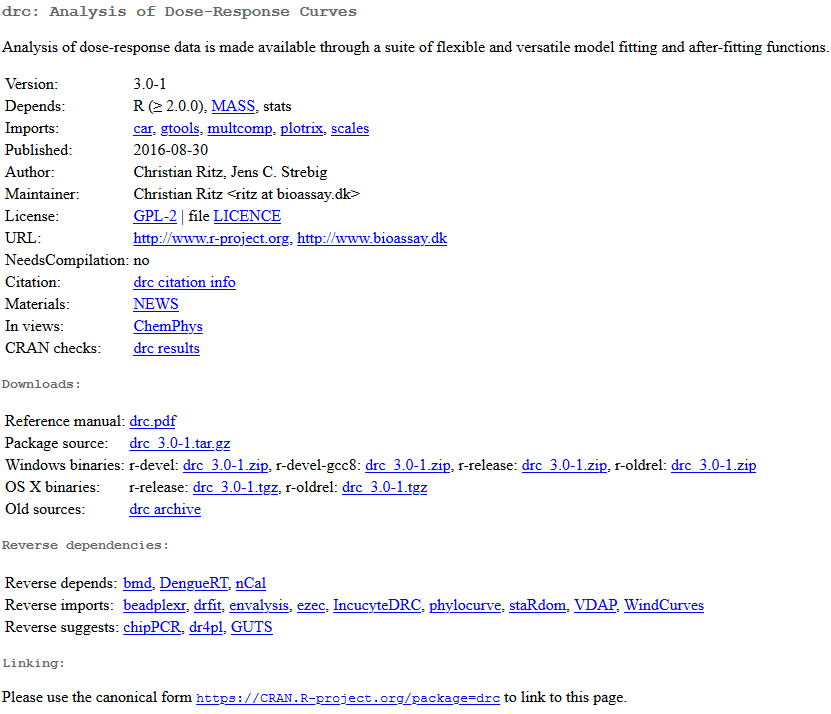
This list can be overwhelming. Go to ‘find’ on your browser and type in ‘drc’. Go through the matched items until you see the package called ‘drc’. Click on it and you’ll see that it’s described as “Analysis of dose-response data is made available through a suite of flexible and versatile model fitting and after-fitting functions.”

There is a lot of information here. The part that’s possibly of the most use is the reference manual in the form of a PDF. Every package in R comes with a reference manual like this, and outlines all of the additional functions and how to use them. We’ll return to this package later.
ggplot2
The first package we’ll use is called ggplot2, where ‘gg’ stands for ‘grammar of graphics’. This is the main plotting tool used in R for producing professional plots.
First, you’ll need to install the package with the following code,
install.packages('ggplot2')
And then load it with,
library('ggplot2')
Let’s take a look at how to use this new package,
elisa = read.csv('../data/data_carpentry_test_data.csv') #Load the data
colnames(elisa) = paste0('Col_', seq(1:13)) #Change the column names

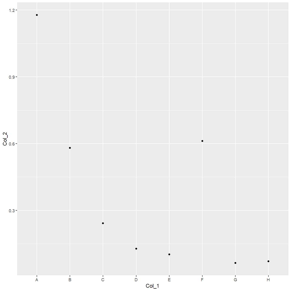
ggplot(data = elisa, aes(x=Col_1, y=Col_2)) +
  geom_point()

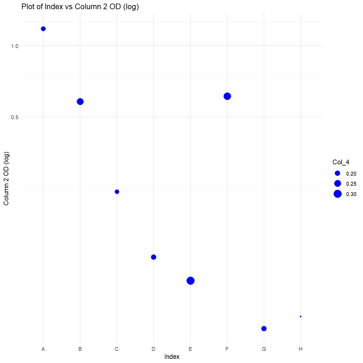
With ggplot, you build up the plot line-by-line.
ggplot(data = elisa, aes(x=Col_1, y=Col_2, size = Col_4)) + #Create the basic plot, of column 1 vs column 2 vs column 3
  geom_point(col = 'blue') + #Create the blue points
  xlab("Index") + #Add an x-label
  ylab("Column 2 OD (log)") + #Add a y-label
  ggtitle("Plot of Index vs Column 2 OD (log)") + #Add a title
  coord_trans(y="log") +
  theme_minimal() #Set to the minimal theme

Exercise: CRAN
Take a look at the CRAN page and manual for ggplot2. Can you apply the function ‘coord_flip()’ to the above code? Have a look in the manual for guidance
Solution
Add '+ coord_flip()' as a new line to the code above
4PL fitting with drc
This section installs and loads the drc package designed for the fitting of standard curves.
Note that this section is aimed at demonstrating the use of external libraries. Don’t worry at this stage if you don’t understand everything that’s going on.
library(drc) #Load the package

elisa_stds = elisa[c(1:5),c(1:3)] #based upon the plate definitions
elisa_stds$standards = c(1000, 500, 250, 125, 62.5) #Add a column of standard values
elisa_stds$log_conc = log10(elisa_stds$standards) #Log the standard values
elisa_stds$OD=rowMeans(elisa_stds[,c(2, 3)], na.rm=TRUE) #Calculate row means for the OD column
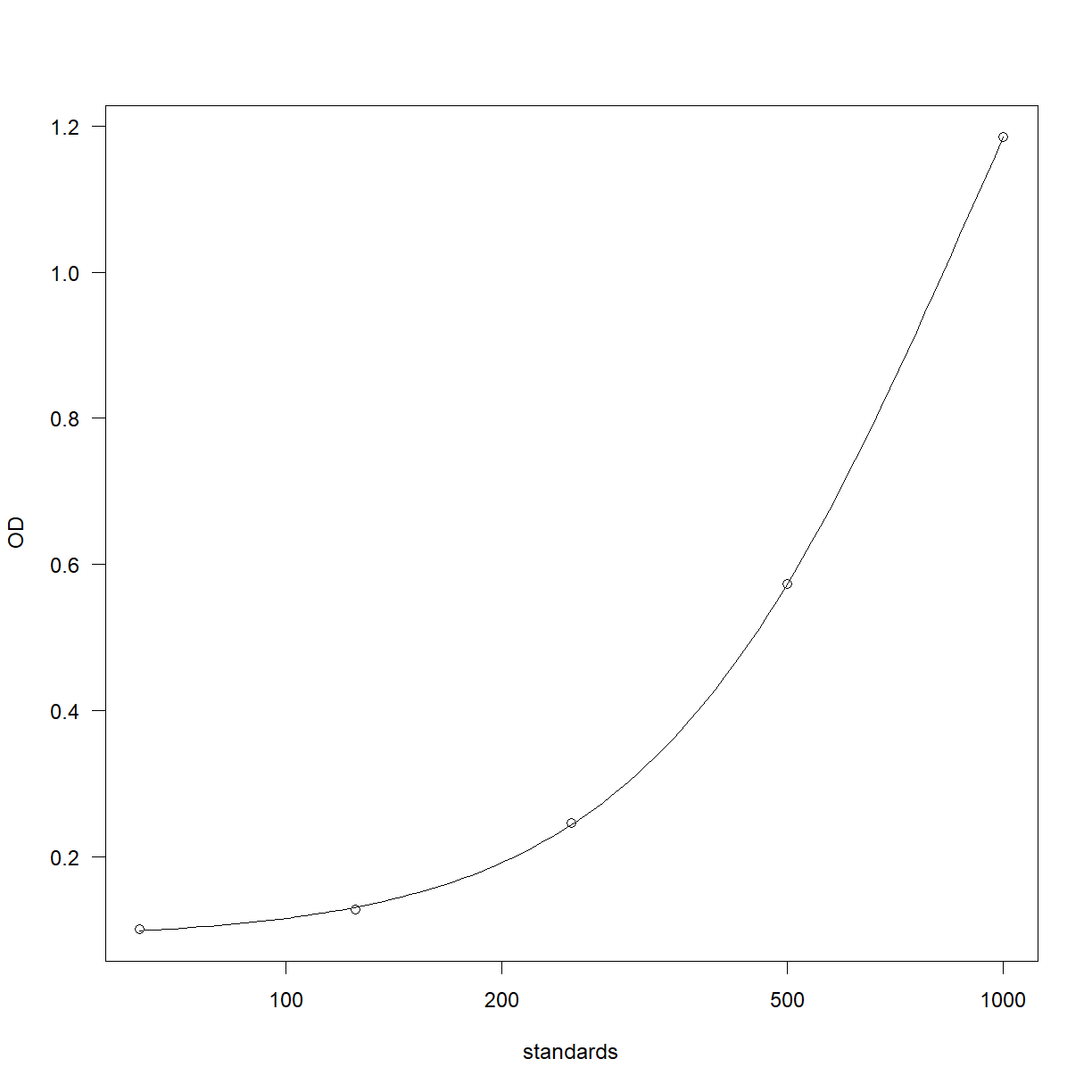
Fit the curve and plot the results,
curve_4pl = drm(OD ~ standards,
            fct=LL.4(),
            data=elisa_stds)

plot(curve_4pl)

Work out the curve backfit and recovery,
elisa_stds$backfit <- ED(curve_4pl, elisa_stds$OD, type="absolute", display=F)
elisa_stds$recovery = (elisa_stds$backfit/elisa_stds$standards)*100
Work out the sample backfits,
Sample_backfits = ED(curve_4pl, c(elisa$Col_4, elisa$Col_5, elisa$Col_6, elisa$Col_7, elisa$Col_8[1:4]), type="absolute", display=T)
Estimated effective doses

          Estimate Std. Error
e:1:0.189 196.4573     3.9012
e:1:0.255 259.6468     6.5999
e:1:0.18  186.7528     3.6861
e:1:0.202 209.8981     4.2991
e:1:0.307 303.4195     9.3673
e:1:0.275 276.9297     7.6276
e:1:0.207 214.9094     4.4755
e:1:0.151 152.4787     3.3986
e:1:0.105  77.8801     3.7311
e:1:0.112  92.5181     3.7271
e:1:0.085       NA         NA
e:1:0.231 237.9525     5.4588
e:1:0.099  63.0539     3.6323
e:1:0.384 363.1657    13.8547
e:1:0.08        NA         NA
e:1:0.229 236.0891     5.3698
e:1:0.116 100.0398     3.6971
e:1:0.074       NA         NA
e:1:0.251 256.1097     6.4017
e:1:0.068       NA         NA
e:1:0.203 210.9069     4.3334
e:1:0.088  18.4156     2.1509
e:1:0.339 328.8090    11.1895
e:1:0.131 124.7666     3.5324
e:1:0.599 517.7610    27.9397
e:1:0.391 368.4000    14.2786
e:1:0.301 298.5464     9.0339
e:1:0.65  554.0446    31.6358
e:1:0.886 730.1957    51.1850
e:1:0.747 624.2809    39.1322
e:1:0.84  694.2439    47.0005
e:1:0.681 576.2718    33.9613
e:1:0.303 300.1752     9.1447
e:1:0.558 488.7158    25.0762
e:1:0.192 199.6157     3.9844
e:1:0.675 571.9565    33.5063
Sample_results = data.frame(Sample_backfits)
Sample_results$Std..Error = NULL
rownames(Sample_results) = seq(1,36)
Sample_results$Marker = paste0('Marker ', seq(1,36))
The coding punchline
We’ve seen a lot of features and functions in R, many of which may seem like they take a significant amount of thought and effort to use. Recall at the start of today the benefits of using code were reproducibililty, efficiency and automation.
The code above, although fairly involved, is completely reproducible. If you were to return to your analysis 18 months from now, you’d be able to see precisely what had been done, starting with the raw data all the way through to the final results.
Next, we’ll see how code like this makes your analysis more efficient, and highlight the automation potential of such code.
First we need to make our own function, to then use like we’ve been using other functions. This is arguably outside the scope of this introduction to R, but the idea is simple to grasp. A function is a chunk of code that takes data in one end, does something to that data, and then returns the processed data. Or, it’s something that does a task such as create a particular plot. The idea behind functions is to limit the amount of repetition in your code. Below is a very simple example,
times_ten = function(number_in) {

  number_out = number_in * 10
  return(number_out)

}
This function, called ‘times_ten’, takes in a number, multiplies it by 10, and then returns the result. Let’s run it,
times_ten(2)
[1] 20
Exercise: Custom functions
Alter the code to instead return the factorial of the entered number (e.g. if the entered number was 4, the result would be 24, as the factorial of 4 is 4 x 3 x 2 x 1). Hint, there is a function for this. Run your code with the number 6. What do you get? Note, call your function ‘factorial_out’. Never give a custom function the same name as a built-in one!
Solution
factorial_out = function(number_in) {

  number_out = factorial(number_in)
  return(number_out)

}

factorial_out(6)

output: [1] 720
One more concept to understand for this lesson are loops. These are for when you want R to repeat a certain section of code, perhaps changing one or more aspects each time. The main loops in R are while loops and for loops. Let’s take a look at a very simple for-loop,
for(i in seq(1:10)) {

  print(paste0('The number is: ', i))

}
[1] "The number is: 1"
[1] "The number is: 2"
[1] "The number is: 3"
[1] "The number is: 4"
[1] "The number is: 5"
[1] "The number is: 6"
[1] "The number is: 7"
[1] "The number is: 8"
[1] "The number is: 9"
[1] "The number is: 10"
Here, we’re asking R to loop through the sequence of numbers, 1 to 10, and for each one, print out the pasted sentence ‘The number is:’ along with ‘i’. In this loop, ‘i’ is the number in the sequence, which increases by 1 each time the loop finishes.
Let’s put this all together. Below is a much larger function that is going to do something very interesting. First, it grabs a list of all the files with a certain keyword in the filename (using the ‘list.files’ function). Then, it goes through each file (using a for-loop), one at a time, performs the 4PL fit, creates a plot, and saves the plot as a png file.
Let’s take a look over the code and the associated comments,
bulk_plots = function(keyword) {

  files = list.files(path = "../data/",
                     pattern = keyword,
                     full.names = T)

  n=1 #for the file number

  #iterate over the files in the directory,
  for (f in files) {

    #read the data,
    elisa = read.csv(f)

    elisa_stds = elisa[c(1:5),c(1:3)] #based upon the plate definitions
    elisa_stds$standards = c(1000, 500, 250, 125, 62.5) #Add a column of standard values
    elisa_stds$log_conc = log10(elisa_stds$standards) #Log the standard values
    elisa_stds$OD=rowMeans(elisa_stds[,c(2, 3)], na.rm=TRUE) #Calculate row means for the OD column

    #fir the curve,
    curve_4pl = drm(OD ~ standards,
                fct=LL.4(),
                data=elisa_stds)

    #save the plot to a png file,
    png(filename = paste0("../data/", 'plot_', n, '_', Sys.Date(), '.png'))

      plot(curve_4pl, col = 'red', main = paste('Plot ', n)) #create the plot

    dev.off() #close the png file
    n=n+1

  }

}
Let’s run it,
bulk_plots('elisa')
Take a look in the folder where the files reside. You should see 10 png files!
Where to go next?
We’ve just seen how to load x10 files, perform x10 curve-fits and produce x10 plots in less than a second. This script could be set to run at a set time each day, if, for example, you had a piece of equipment that was generating raw data files on a regular basis.
Of course, mistakes can still be made when using code instead of mouse-clicks, but crucially, these mistakes are much easier to spot. For very important work, consider getting a colleague to review your code.
R can generate not only images, but processed data-files, mathematical models, full reports in Word or PDF formats, slides, websites and even interactive apps. The level of sophistication is unlimited and can make any routine data processes much quicker, transparent and less prone to human copy-and-paste errors. Any process that you have in your department or company that’s done on a regular basis could and should be performed by code.
Good luck on your R journey!
Key Points
R can be extended in thousands of different ways