Introduction

Overview

Teaching: 20 min
Exercises: 5 min

Questions

• What problems are we solving, and what are we not discussing?

• Why do we use Python?

• What is parallel programming?

• Why can it be hard to write a parallel program?

Objectives

• Recognize serial and parallel patterns

• Identify problems that can be parallelized

• Understand a dependency diagram

Common problems

What problems are we solving?

Ask around what problems participants encountered: “Why did you sign up?”. Specifically: what is the domain science related task that you want to parallelize?

Most problems will fit in one of two categories:

• I wrote this code in Python and it is not fast enough.
• I run this code on my laptop, but the target problem size is bigger than the RAM.

In this course we will show several possible ways of speeding up your program and making it ready to function in parallel. We will be introducing the following modules:

1. threading allows different parts of your program to run concurrently on a single computer (with shared memory)
2. dask makes scalable parallel computing easy
3. numba speeds up your Python functions by translating them to optimized machine code
4. memory_profile monitors memory performance
5. asyncio Python’s native asynchronous programming

FIXME: Actually explain functional programming & distributed programming More importantly, we will show how to change the design of a program to fit parallel paradigms. This often involves techniques from functional programming.

What we won’t talk about

In this course we will not talk about distributed programming. This is a huge can of worms. It is easy to show simple examples, but depending on the problem, solutions will be wildly different. Dask has a lot of functionality to help you in setting up for running on a network. The important bit is that, once you have made your code suitable for parallel computing, you’ll have the right mind-set to get it to work in a distributed environment.

Overview and rationale

This is an advanced course. Why is it advanced? We (hopefully) saw in the discussion that although many of your problems share similar characteristics, it is the detail that will determine the solution. We all need our algorithms, models, analysis to run in a way that many hands make light work. When such a situation arises with a group of people, we start with a meeting discussing who does what, when do we meet again to sync up, etc. After a while you can get the feeling that all you do is be in meetings. We will see that there are several abstractions that can make our life easier. In large parts this course will use Dask to illustrate these abstractions.

• Vectorized instructions: tell many workers to do the same work on a different piece of data. This is where dask.array and dask.dataframe come in. We will illustrate this model of working by computing the number Pi later on.
• Map/filter/reduce: this is a method where we combine different functionals to create a larger program. We will use dask.bag to count the number of unique words in a novel using this formalism.
• Task-based parallelization: this may be the most generic abstraction as all the others can be expressed in terms of tasks or workflows. This is dask.delayed.

Why Python?

Python is one of most widely used languages to do scientific data analysis, visualization, and even modelling and simulation. The popularity of Python is mainly due to the two pillars of a friendly syntax together with the availability of many high-quality libraries.

It’s not all good news

The flexibility that Python offers comes with a few downsides though:

• Python code typically doesn’t perform as fast as lower-level implementations in C/C++ or Fortran.
• It is not trivial to parallelize Python code to work efficiently on many-core architectures.

This workshop addresses both these issues, with an emphasis on being able to run Python code efficiently (in parallel) on multiple cores.

What is parallel computing?

Dependency diagrams

Suppose we have a computation where each step depends on a previous one. We can represent this situation like in the figure below, known as a dependency diagram:

In these diagrams the inputs and outputs of each function are represented as rectangles. The inward and outward arrows indicate their flow. Note that the output of one function can become the input of another one. The diagram above is the typical diagram of a serial computation. If you ever used a loop to update a value, you used serial computation.

If our computation involves independent work (that is, the results of the application of each function are independent of the results of the application of the rest), we can structure our computation like this:

This scheme corresponds to a parallel computation.

How can parallel computing improve our code execution speed?

Nowadays, most personal computers have 4 or 8 processors (also known as cores). In the diagram above, we can assign each of the three functions to one core, so they can be performed simultaneously.

Do 8 processors work 8 times faster than one?

It may be tempting to think that using eight cores instead of one would multiply the execution speed by eight. For now, it’s ok to use this a first approximation to reality. Later in the course we’ll see that things are actually more complicated than that.

Parallelizable and non-parallelizable tasks

Some tasks are easily parallelizable while others inherently aren’t. However, it might not always be immediately apparent that a task is parallelizable.

FIXME: this may be too much

Let us consider the following piece of code.

x = [1, 2, 3, 4] # Write input

y = 0 # Initialize output

for i in range(len(x)):
  y += x[i] # Add each element to the output variable

print(y) # Print output

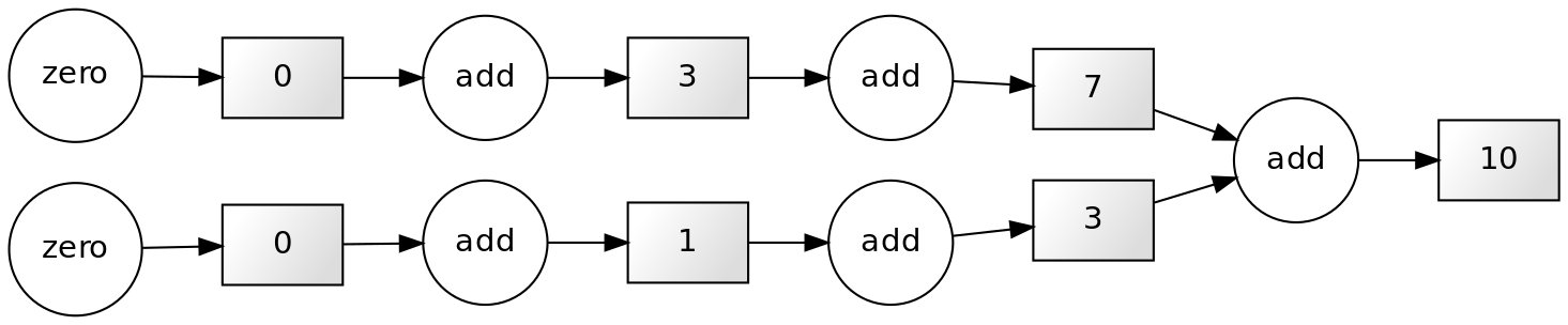
Note that each successive loop uses the result of the previous loop. In that way, it is dependent on the previous loop. The following dependency diagram makes that clear:

Although we are performing the loops in a serial way in the snippet above, nothing avoids us from performing this calculation in parallel. The following example shows that parts of the computations can be done independently:

x = [1, 2, 4, 4]

chunk1 = x[:2]
chunk2 = x[2:]

sum_1 = sum(chunk1)
sum_2 = sum(chunk2)

result = sum_1 + sum_2

print(result)

The technique for parallelising sums like this is called chunking.

There is a subclass of algorithms where the subtasks are completely independent. These kinds of algorithms are known as embarrassingly parallel, or more friendly naturally or delightfully parallel.

An example of this kind of problem is squaring each element in a list, which can be done like so:

y = [n**2 for n in x]

Each task of squaring a number is independent of all the other elements in the list.

It is important to know that some tasks are fundamentally non-parallelizable. An example of such an inherently serial algorithm could be the computation of the fibonacci sequence using the formula Fn=Fn-1 + Fn-2. Each output here depends on the outputs of the two previous loops.

Challenge: Parallellizable and non-parallellizable tasks

Can you think of a task in your domain that is parallelizable? Can you also think of one that is fundamentally non-parallelizable?

Please write your answers in the collaborative document.

Problems versus Algorithms

Often, the parallelizability of a problem depends on its specific implementation. For instance, in our first example of a non-parallelizable task, we mentioned the calculation of the Fibonacci sequence. However, there exists a closed form expression to compute the n-th Fibonacci number.

Last but not least, don’t let the name demotivate you: if your algorithm happens to be embarrassingly parallel, that’s good news! The “embarrassingly” refers to the feeling of “this is great!, how did I not notice before?!”

Challenge: Parallelised Pea Soup

We have the following recipe:

1. (1 min) Pour water into a soup pan, add the split peas and bay leaf and bring it to boil.
2. (60 min) Remove any foam using a skimmer and let it simmer under a lid for about 60 minutes.
3. (15 min) Clean and chop the leek, celeriac, onion, carrot and potato.
4. (20 min) Remove the bay leaf, add the vegetables and simmer for 20 more minutes. Stir the soup occasionally.
5. (1 day) Leave the soup for one day. Reheat before serving and add a sliced smoked sausage (vegetarian options are also welcome). Season with pepper and salt.

Imagine you’re cooking alone.

• Can you identify potential for parallelisation in this recipe?
• And what if you are cooking with the help of a friend help? Is the soup done any faster?
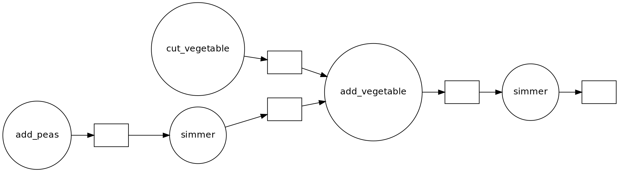
• Draw a dependency diagram.

Solution

• You can cut vegetables while simmering the split peas.
• If you have help, you can parallelize cutting vegetables further.
• There are two ‘workers’: the cook and the stove.

Shared vs. Distributed memory

FIXME: add text

Key Points

• Programs are parallelizable if you can identify independent tasks.

• To make programs scalable, you need to chunk the work.

• Parallel programming often triggers a redesign; we use different patterns.

• Doing work in parallel does not always give a speed-up.

Measuring performance

Overview

Teaching: 40 min
Exercises: 20 min

Questions

• How do we know our program ran faster?

• How do we learn about efficiency?

Objectives

• View performance on system monitor

• Find out how many cores your machine has

• Use %time and %timeit line-magic

• Use a memory profiler

• Plot performance against number of work units

• Understand the influence of hyper-threading on timings

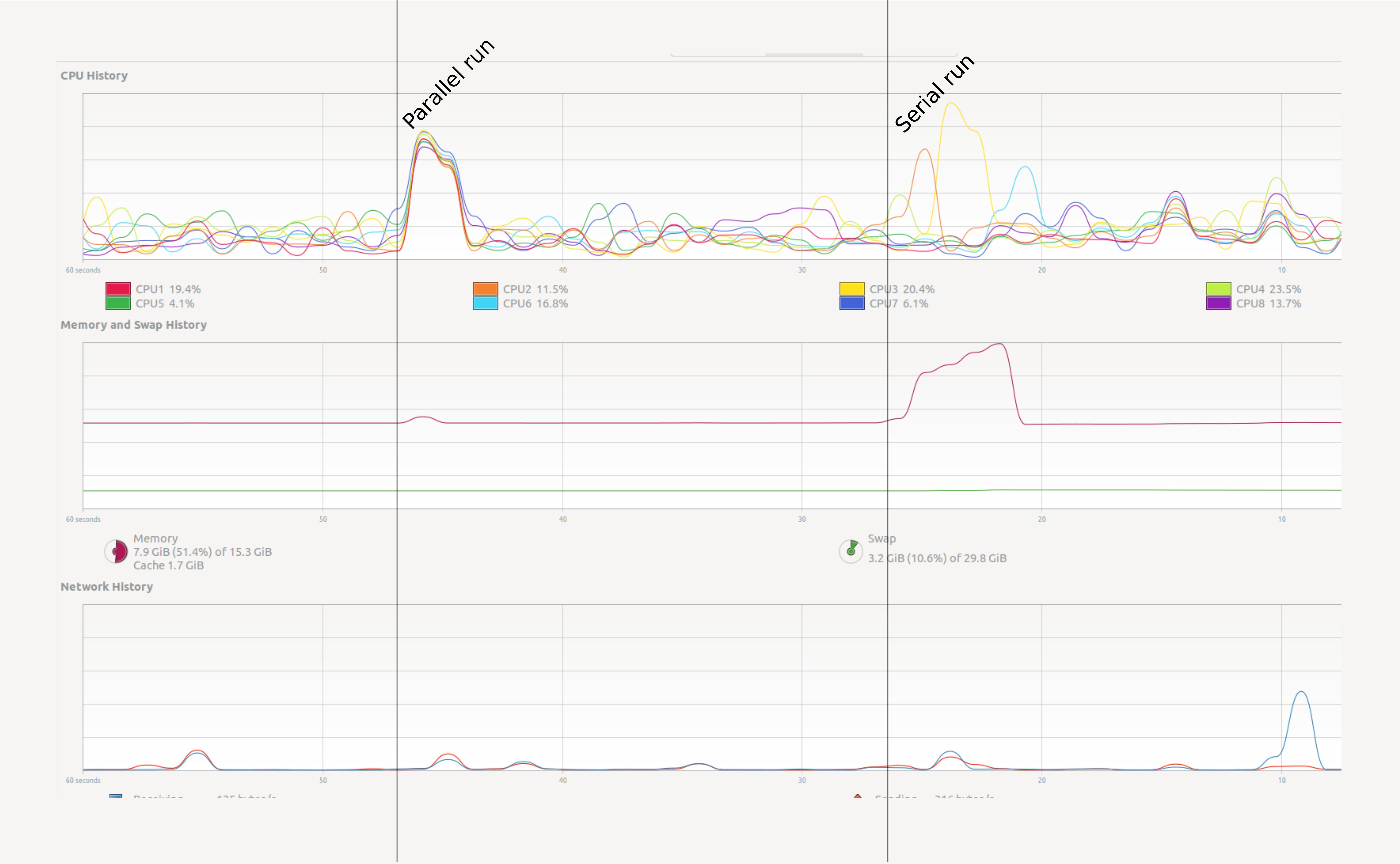
A first example with Dask

We will get into creating parallel programs in Python later. First let’s see a small example. Open your system monitor (this will differ among specific operating systems), and run the following code examples.

# Summation making use of numpy:
import numpy as np
result = np.arange(10**7).sum()

# The same summation, but using dask to parallelize the code.
# NB: the API for dask arrays mimics that of numpy
import dask.array as da
work = da.arange(10**7).sum()
result = work.compute()

Try a heavy enough task

It could be that a task this small does not register on your radar. Depending on your computer you will have to raise the power to 10**8 or 10**9 to make sure that it runs long enough to observe the effect. But be careful and increase slowly. Asking for too much memory can make your computer slow to a crawl.

How can we test this in a more practical way? In Jupyter we can use some line magics, small “magic words” preceded by the symbol %% that modify the behaviour of the cell.

%%time
np.arange(10**7).sum()

The %%time line magic checks how long it took for a computation to finish. It does nothing to change the computation itself. In this it is very similar to the time shell command.

If run the chunk several times, we will notice a difference in the times. How can we trust this timer, then? A possible solution will be to time the chunk several times, and take the average time as our valid measure. The %%timeit line magic does exactly this in a concise an comfortable manner! %%timeit first measures how long it takes to run a command one time, then repeats it enough times to get an average run-time. Also, %%timeit can measure run times without the time it takes to setup a problem, measuring only the performance of the code in the cell. This way we can trust the outcome better.

%%timeit
np.arange(10**7).sum()

If you want to store the output of %%timeit in a Python variable, you can do so with the -o flag.

time = %timeit -o np.arange(10**7).sum()
print(f"Time taken: {time.average:.4f}s")

Note that this does not tell you anything about memory consumption or efficiency.

Memory profiling

• The act of systematically testing performance under different conditions is called benchmarking.
• Analysing what parts of a program contribute to the total performance, and identifying possible bottlenecks is profiling.

We will use the memory_profiler package to track memory usage. It can be installed executing the code below in the console:

pip install memory_profiler

In Jupyter, type the following lines to compare the memory usage of the serial and parallel versions of the code presented above (again, change the value of 10**7 to something higher if needed):

import numpy as np
import dask.array as da
from memory_profiler import memory_usage
import matplotlib.pyplot as plt

def sum_with_numpy():
    # Serial implementation
    np.arange(10**7).sum()

def sum_with_dask():
    # Parallel implementation
    work = da.arange(10**7).sum()
    work.compute()

memory_numpy = memory_usage(sum_with_numpy, interval=0.01)
memory_dask = memory_usage(sum_with_dask, interval=0.01)

# Plot results
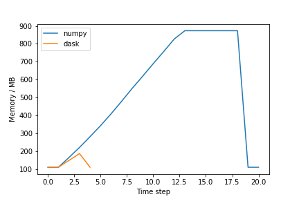
plt.plot(memory_numpy, label='numpy')
plt.plot(memory_dask, label='dask')
plt.xlabel('Time step')
plt.ylabel('Memory / MB')
plt.legend()
plt.show()

The figure should be similar to the one below:

Exercise (plenary)

Why is the Dask solution more memory efficient?

Solution

Chunking! Dask chunks the large array, such that the data is never entirely in memory.

Profiling from Dask

Dask has several option to do profiling from Dask itself. See the dask documentation for more information.

Using many cores

Using more cores for a computation can decrease the run time. The first question is of course: how many cores do I have? See the snippets below to find out:

Find out how many cores your machine has

The number of cores can be found from Python by executing:

import psutil
N_physical_cores = psutil.cpu_count(logical=False)
N_logical_cores = psutil.cpu_count(logical=True)
print(f"The number of physical/logical cores is {N_physical_cores}/{N_logical_cores}")

Usually the number of logical cores is higher than the number of physical course. This is due to hyper-threading, which enables each physical CPU core to execute several threads at the same time. Even with simple examples, performance may scale unexpectedly. There are many reasons for this, hyper-threading being one of them.

See for instance the example below:

On a machine with 4 physical and 8 logical cores doing this (admittedly oversimplistic) benchmark:

x = []
for n in range(1, 9):
    time_taken = %timeit -r 1 -o da.arange(5*10**7).sum().compute(num_workers=n)
    x.append(time_taken.average)

Gives the following result:

import pandas as pd
data = pd.DataFrame({"n": range(1, 9), "t": x})
data.set_index("n").plot()

Discussion

Why is the runtime increasing if we add more than 4 cores? This has to do with hyper-threading. On most architectures it does not make much sense to use more workers than the number of physical cores you have.

Key Points

• It is often non-trivial to understand performance

• Memory is just as important as speed

• Measuring is knowing

Accellerators: vectorized Numpy and Numba

Overview

Teaching: 60 min
Exercises: 30 min

Questions

• How do I parallelize a Python application?

• What is data parallelism?

• What is task parallelism?

Objectives

• Rewrite a program in a vectorized form.

• Understand the difference between data and task-based parallel programming.

• Apply numba.jit to accelerate Python.

Parallelizing a Python application

In order to recognize the advantages of parallelization we need an algorithm that is easy to parallelize, but still complex enough to take a few seconds of CPU time. To not scare away the interested reader, we need this algorithm to be understandable and, if possible, also interesting. We chose a classical algorithm for demonstrating parallel programming: estimating the value of number π.

The algorithm we present is one of the classical examples of the power of Monte-Carlo methods. This is an umbrella term for several algorithms that use random numbers to approximate exact results. We chose this algorithm because of its simplicity and straightforward geometrical interpretation.

We can compute the value of π using a random number generator. We count the points falling inside the blue circle M compared to the green square N. Then π is approximated by the ratio 4M/N.

Challenge: Implement the algorithm

Use only standard Python and the function random.uniform. The function should have the following interface:

import random
def calc_pi(N):
    """Computes the value of pi using N random samples."""
    ...
    for i in range(N):
        # take a sample
        ...
    return ...

Also make sure to time your function!

Solution

import random

def calc_pi(N):
    M = 0
    for i in range(N):
        # Simulate impact coordinates
        x = random.uniform(-1, 1)
        y = random.uniform(-1, 1)

        # True if impact happens inside the circle
        if x**2 + y**2 < 1.0:
            M += 1
    return 4 * M / N

%timeit calc_pi(10**6)

676 ms ± 6.39 ms per loop (mean ± std. dev. of 7 runs, 1 loop each)

Before we start to parallelize this program, we need to do our best to make the inner function as efficient as we can. We show two techniques for doing this: vectorization using numpy and native code generation using numba.

We first demonstrate a Numpy version of this algorithm.

import numpy as np

def calc_pi_numpy(N):
    # Simulate impact coordinates
    pts = np.random.uniform(-1, 1, (2, N))
    # Count number of impacts inside the circle
    M = np.count_nonzero((pts**2).sum(axis=0) < 1)
    return 4 * M / N

This is a vectorized version of the original algorithm. It nicely demonstrates data parallelization, where a single operation is replicated over collections of data. It contrasts to task parallelization, where different independent procedures are performed in parallel (think for example about cutting the vegetables while simmering the split peas).

If we compare with the ‘naive’ implementation above, we see that our new one is much faster:

%timeit calc_pi_numpy(10**6)

25.2 ms ± 1.54 ms per loop (mean ± std. dev. of 7 runs, 10 loops each)

Discussion: is this all better?

What is the downside of the vectorized implementation?

• It uses more memory
• It is less intuitive
• It is a more monolithic approach, i.e. you cannot break it up in several parts

Challenge: Daskify

Write calc_pi_dask to make the Numpy version parallel. Compare speed and memory performance with the Numpy version. NB: Remember that dask.array mimics the numpy API.

Solution

import dask.array as da

def calc_pi_dask(N):
    # Simulate impact coordinates
    pts = da.random.uniform(-1, 1, (2, N))
    # Count number of impacts inside the circle
    M = da.count_nonzero((pts**2).sum(axis=0) < 1)
    return 4 * M / N

%timeit calc_pi_dask(10**6).compute()

4.68 ms ± 135 µs per loop (mean ± std. dev. of 7 runs, 100 loops each)

Using Numba to accelerate Python code

Numba makes it easier to create accelerated functions. You can use it with the decorator numba.jit.

import numba

@numba.jit
def sum_range_numba(a):
    """Compute the sum of the numbers in the range [0, a)."""
    x = 0
    for i in range(a):
        x += i
    return x

Let’s time three versions of the same test. First, native Python iterators:

%timeit sum(range(10**7))

190 ms ± 3.26 ms per loop (mean ± std. dev. of 7 runs, 10 loops each)

Now with Numpy:

%timeit np.arange(10**7).sum()

17.5 ms ± 138 µs per loop (mean ± std. dev. of 7 runs, 100 loops each)

And with Numba:

%timeit sum_range_numba(10**7)

162 ns ± 0.885 ns per loop (mean ± std. dev. of 7 runs, 10000000 loops each)

Numba is 100x faster in this case! It gets this speedup with “just-in-time” compilation (JIT)—compiling the Python function into machine code just before it is called (that’s what the @numba.jit decorator stands for). Not every Python and Numpy feature is supported, but a function may be a good candidate for Numba if it is written with a Python for-loop over a large range of values, as with sum_range_numba().

Just-in-time compilation speedup

The first time you call a function decorated with @numba.jit, you may see little or no speedup. In subsequent calls, the function could be much faster. You may also see this warning when using timeit:

The slowest run took 14.83 times longer than the fastest. This could mean that an intermediate result is being cached.

Why does this happen? On the first call, the JIT compiler needs to compile the function. On subsequent calls, it reuses the already-compiled function. The compiled function can only be reused if it is called with the same argument types (int, float, etc.).

See this example where sum_range_numba is timed again, but now with a float argument instead of int:

%time sum_range_numba(10.**7)
%time sum_range_numba(10.**7)

CPU times: user 58.3 ms, sys: 3.27 ms, total: 61.6 ms
Wall time: 60.9 ms
CPU times: user 5 µs, sys: 0 ns, total: 5 µs
Wall time: 7.87 µs

Challenge: Numbify calc_pi

Create a Numba version of calc_pi. Time it.

Solution

Add the @numba.jit decorator to the first ‘naive’ implementation.

@numba.jit
def calc_pi_numba(N):
    M = 0
    for i in range(N):
        # Simulate impact coordinates
        x = random.uniform(-1, 1)
        y = random.uniform(-1, 1)

        # True if impact happens inside the circle
        if x**2 + y**2 < 1.0:
            M += 1
    return 4 * M / N

%timeit calc_pi_numba(10**6)

13.5 ms ± 634 µs per loop (mean ± std. dev. of 7 runs, 1 loop each)

Measuring == knowing

Always profile your code to see which parallelization method works best.

numba.jit is not a magical command to solve are your problems

Using numba to accelerate your code often outperforms other methods, but it is not always trivial to rewrite your code so that you can use numba with it.

Key Points

• Always profile your code to see which parallelization method works best

• Vectorized algorithms are both a blessing and a curse.

• Numba can help you speed up code

Dask abstractions: delays

Overview

Teaching: 60 min
Exercises: 30 min

Questions

• What abstractions does Dask offer?

• What programming patterns exist in the parallel universe?

Objectives

• Understand the abstraction of delayed evaluation

• Use the visualize method to create dependency graphs

Dask is one of the many tools available for parallelizing Python code in a comfortable way. We’ve seen a basic example of dask.array in a previous episode. Now, we will focus on the delayed and bag sub-modules. Dask has a lot of other useful components, such as dataframe and futures, but we are not going to cover them in this lesson.

See an overview below:

Dask Delayed

A lot of the functionality in Dask is based on top of a framework of delayed evaluation. The concept of delayed evaluation is very important in understanding how Dask functions, which is why we will go a bit deeper into dask.delayed.

from dask import delayed

The delayed decorator builds a dependency graph from function calls.

@delayed
def add(a, b):
    result = a + b
    print(f"{a} + {b} = {result}")
    return a + b

A delayed function stores the requested function call inside a promise. The function is not actually executed yet, instead we are promised a value that can be computed later.

x_p = add(1, 2)

We can check that x_p is now a Delayed value.

type(x_p)

[out]: dask.delayed.Delayed

Note

It is often a good idea to suffix variables that you know are promises with _p. That way you keep track of promises versus immediate values.

Only when we evaluate the computation, do we get an output.

x_p.compute()

1 + 2 = 3
[out]: 3

From Delayed values we can create larger workflows and visualize them.

x_p = add(1, 2)
y_p = add(x_p, 3)
z_p = add(x_p, y_p)
z_p.visualize(rankdir="LR")

Challenge: run the workflow

Given this workflow:

x_p = add(1, 2)
y_p = add(x_p, 3)
z_p = add(x_p, -3)

Visualize and compute y_p and z_p, how often is x_p evaluated? Now change the workflow:

x_p = add(1, 2)
y_p = add(x_p, 3)
z_p = add(x_p, y_p)
z_p.visualize(rankdir="LR")

We pass the yet uncomputed promise x_p to both y_p and z_p. How often do you expect x_p to be evaluated? Run the workflow to check your answer.

Solution

z_p.compute()

1 + 2 = 3
3 + 3 = 6
3 + 6 = 9
[out]: 9

The computation of x_p (1 + 2) appears only once.

We can also make a promise by directly calling delayed

N = 10**7
x_p = delayed(calc_pi)(N)

It is now possible to call visualize or compute methods on x_p.

Variadic arguments

In Python you can define functions that take arbitrary number of arguments:

def add(*args):
 return sum(args)

add(1, 2, 3, 4)   # => 10

You can use tuple-unpacking to pass a sequence of arguments:

numbers = [1, 2, 3, 4]
add(*numbers)   # => 10

We can build new primitives from the ground up.

@delayed
def gather(*args):
    return list(args)

Challenge: understand gather

Can you describe what the gather function does in terms of lists and promises?

Solution

It turns a list of promises into a promise of a list.

We can visualize what gather does by this small example.

x_p = gather(*(add(n, n) for n in range(10))) # Shorthand for gather(add(1, 1), add(2, 2), ...)
x_p.visualize()

Computing the result,

x_p.compute()

[out]: [0, 1, 4, 9, 16, 25, 36, 49, 64, 81]

Challenge: design a mean function and calculate pi

Write a delayed function that computes the mean of its arguments. Use it to esimates pi several times and returns the mean of the results.

>>> mean(1, 2, 3, 4).compute()
2.5

Make sure that the entire computation is contained in a single promise.

Solution

from dask import delayed
import random

@delayed
def mean(*args):
    return sum(args) / len(args)

def calc_pi(N):
    """Computes the value of pi using N random samples."""
    M = 0
    for i in range(N):
        # take a sample
        x = random.uniform(-1, 1)
        y = random.uniform(-1, 1)
        if x*x + y*y < 1.: M+=1
    return 4 * M / N


N = 10**6
pi_p = mean(*(delayed(calc_pi)(N) for i in range(10)))
pi_p.compute()

You may not seed a significant speedup. This is because dask delayed uses threads by default and our native Python implementation of calc_pi does not circumvent the GIL. With for example the numba version of calc_pi you should see a more significant speedup.

In practice you may not need to use @delayed functions too often, but it does offer ultimate flexibility. You can build complex computational workflows in this manner, sometimes replacing shell scripting, make files and the likes.

Key Points

• Use abstractions to keep programs manageable

Threading and Multiprocessing

Overview

Teaching: 60 min
Exercises: 30 min

Questions

• What is the Global Interpreter Lock (GIL)?

• How do I use multiple threads in Python?

Objectives

• Understand the GIL.

• Understand the difference between the python threading and multiprocessing library

Threading

Another possibility for parallelization is to use the threading module. This module is built into Python. In this section, we’ll use it to estimate pi once again.

Using threading to speed up your code:

from threading import (Thread)

%%time
n = 10**7
t1 = Thread(target=calc_pi, args=(n,))
t2 = Thread(target=calc_pi, args=(n,))

t1.start()
t2.start()

t1.join()
t2.join()

Discussion: where’s the speed-up?

While mileage may vary, parallelizing calc_pi, calc_pi_numpy and calc_pi_numba this way will not give the expected speed-up. calc_pi_numba should give some speed-up, but nowhere near the ideal scaling over the number of cores. This is because Python only allows one thread to access the interperter at any given time, a feature also known as the Global Interpreter Lock.

A few words about the Global Interpreter Lock

The Global Interpreter Lock (GIL) is an infamous feature of the Python interpreter. It both guarantees inner thread sanity, making programming in Python safer, and prevents us from using multiple cores from a single Python instance. When we want to perform parallel computations, this becomes an obvious problem. There are roughly two classes of solutions to circumvent/lift the GIL:

• Run multiple Python instances: multiprocessing
• Have important code outside Python: OS operations, C++ extensions, cython, numba

The downside of running multiple Python instances is that we need to share program state between different processes. To this end, you need to serialize objects. Serialization entails converting a Python object into a stream of bytes, that can then be sent to the other process, or e.g. stored to disk. This is typically done using pickle, json, or similar, and creates a large overhead. The alternative is to bring parts of our code outside Python. Numpy has many routines that are largely situated outside of the GIL. The only way to know for sure is trying out and profiling your application.

To write your own routines that do not live under the GIL there are several options: fortunately numba makes this very easy.

We can force the GIL off in Numba code by setting nogil=True in the numba.jit decorator.

@numba.jit(nopython=True, nogil=True)
def calc_pi_nogil(N):
    M = 0
    for i in range(N):
        x = random.uniform(-1, 1)
        y = random.uniform(-1, 1)
        if x**2 + y**2 < 1:
            M += 1
    return 4 * M / N

The nopython argument forces Numba to compile the code without referencing any Python objects, while the nogil argument enables lifting the GIL during the execution of the function.

Use nopython=True or @numba.njit

It’s generally a good idea to use nopython=True with @numba.jit to make sure the entire function is running without referencing Python objects, because that will dramatically slow down most Numba code. There’s even a decorator that has nopython=True by default: @numba.njit

Now we can run the benchmark again, using calc_pi_nogil instead of calc_pi.

Exercise: try threading on a Numpy function

Many Numpy functions unlock the GIL. Try to sort two randomly generated arrays using numpy.sort in parallel.

Solution

rnd1 = np.random.random(high)
rnd2 = np.random.random(high)
%timeit -n 10 -r 10 np.sort(rnd1)

%%timeit -n 10 -r 10
t1 = Thread(target=np.sort, args=(rnd1, ))
t2 = Thread(target=np.sort, args=(rnd2, ))

t1.start()
t2.start()

t1.join()
t2.join()

Multiprocessing

Python also allows for using multiple processes for parallelisation via the multiprocessing module. It implements an API that is superficially similar to threading:

from multiprocessing import Process

def calc_pi(N):
    ...

if __name__ == '__main__':
    n = 10**7
    p1 = Process(target=calc_pi, args=(n,))
    p2 = Process(target=calc_pi, args=(n,))

    p1.start()
    p2.start()

    p1.join()
    p2.join()

However under the hood processes are very different from threads. A new process is created by creating a fresh “copy” of the python interpreter, that includes all the resources associated to the parent. There are three different ways of doing this (spawn, fork, and forkserver), which depends on the platform. We will use spawn as it is available on all platforms, you can read more about the others in the Python documentation. As creating a process is resource intensive, multiprocessing is beneficial under limited circumstances - namely, when the resource utilisation (or runtime) of a function is measureably larger than the overhead of creating a new process.

Protect process creation with an if-block

A module should be safely importable. Any code that creates processes, pools, or managers should be protected with:

if __name__ == "__main__":
    ...

The non-intrusive and safe way of starting a new process is acquire a context, and working within the context. This ensures your application does not interfere with any other processes that might be in use.

import multiprocessing as mp


def calc_pi(N):
    ...

if __name__ == '__main__':
    # mp.set_start_method("spawn")  # if not using a context
    ctx = mp.get_context("spawn")
	...

Passing objects and sharing state

We can pass objects between processes by using Queues and Pipes. Multiprocessing queues behave similarly to regular queues:

• FIFO: first in, first out
• queue_instance.put(<obj>) to add
• queue_instance.get() to retrieve

Exercise: reimplement calc_pi to use a queue to return the result

Solution

import multiprocessing as mp
import random


def calc_pi(N, que):
    M = 0
    for i in range(N):
        # Simulate impact coordinates
        x = random.uniform(-1, 1)
        y = random.uniform(-1, 1)

        # True if impact happens inside the circle
        if x**2 + y**2 < 1.0:
            M += 1
    que.put((4 * M / N, N))  # result, iterations


if __name__ == "__main__":
    ctx = mp.get_context("spawn")
    que = ctx.Queue()
    n = 10**7
    p1 = ctx.Process(target=calc_pi, args=(n, que))
    p2 = ctx.Process(target=calc_pi, args=(n, que))
    p1.start()
    p2.start()

    for i in range(2):
        print(que.get())

    p1.join()
    p2.join()

Sharing state

It is also possible to share state between processes. The simpler of the several ways is to use shared memory via Value or Array. You can access the underlying value using the .value property. Note, in case you want to do an operation that is not atomic (cannot be done in one step, e.g. using the += operator), you should explicitly acquire a lock before performing the operation:

with var.get_lock():
    var.value += 1

Since Python 3.8, you can also create a numpy array backed by a shared memory buffer (multiprocessing.shared_memory.SharedMemory), which can then be accessed from separate processes by name (including separate interactive shells!).

Process pool

The Pool API provides a pool of worker processes that can execute tasks. Methods of the pool object offer various convenient ways to implement data parallelism in your program. The most convenient way to create a pool object is with a context manager, either using the toplevel function multiprocessing.Pool, or by calling the .Pool() method on the context. With the pool object, tasks can be submitted by calling methods like .apply(), .map(), .starmap(), or their .*_async() versions.

Exercise: adapt the original exercise to submit tasks to a pool

• Use the original calc_pi function (without the queue)
• Submit batches of different sample size (different values of N).
• As mentioned earlier, creating a new process has overhead. Try a wide range of sample sizes and check if runtime scaling supports that claim.

Solution

from itertools import repeat
import multiprocessing as mp
import random
from timeit import timeit


def calc_pi(N):
    M = 0
    for i in range(N):
        # Simulate impact coordinates
        x = random.uniform(-1, 1)
        y = random.uniform(-1, 1)

        # True if impact happens inside the circle
        if x**2 + y**2 < 1.0:
            M += 1
    return (4 * M / N, N)  # result, iterations


def submit(ctx, N):
    with ctx.Pool() as pool:
        pool.starmap(calc_pi, repeat((N,), 4))


if __name__ == "__main__":
    ctx = mp.get_context("spawn")
    for i in (1_000, 100_000, 10_000_000):
        res = timeit(lambda: submit(ctx, i), number=5)
        print(i, res)

Key Points

• If we want the most efficient parallelism on a single machine, we need to circumvent the GIL.

• If your code releases the GIL, threading will be more efficient than multiprocessing.

Dask abstractions: bags

Overview

Teaching: 60 min
Exercises: 30 min

Questions

• What abstractions does Dask offer?

• What programming patterns exist in the parallel universe?

Objectives

• Recognize map, filter and reduce patterns

• Create programs using these building blocks

• Use the visualize method to create dependency graphs

Dask bags let you compose functionality using several primitive patterns: the most important of these are map, filter, groupby and reduce.

Discussion

Open the Dask documentation on bags. Discuss the map and filter and reduction methods

Operations on this level can be distinguished in several categories:

• map (N to N) applies a function one-to-one on a list of arguments. This operation is embarrassingly parallel.
• filter (N to <N) selects a subset from the data.
• groupby (N to <N) groups data in subcategories.
• reduce (N to 1) computes an aggregate from a sequence of data; if the operation permits it (summing, maximizing, etc) this can be done in parallel by reducing chunks of data and then further processing the results of those chunks.

Let’s see an example of it in action:

First, let’s create the bag containing the elements we want to work with (in this case, the numbers from 0 to 5).

import dask.bag as db

bag = db.from_sequence(['mary', 'had', 'a', 'little', 'lamb'])

Map

To illustrate the concept of map, we’ll need a mapping function. In the example below we’ll just use a function that squares its argument:

# Create a function for mapping
def f(x):
    return x.upper()

# Create the map and compute it
bag.map(f).compute()

out: ['MARY', 'HAD', 'A', 'LITTLE', 'LAMB']

We can also visualize the mapping:

# Visualize the map
bag.map(f).visualize()

Filter

To illustrate the concept of filter, it is useful to have a function that returns a boolean. In this case, we’ll use a function that returns True if the argument contains the letter ‘a’, and False if it doesn’t.

# Return True if x is even, False if not
def pred(x):
    return 'a' in x

bag.filter(pred).compute()

[out]: ['mary', 'had', 'a', 'lamb']

Difference between filter and map

Without executing it, try to forecast what would be the output of bag.map(pred).compute().

Solution

The output will be [True, True, True, False, True].

Reduction

def count_chars(x):
    per_word = [len(w) for w in x]

    return sum(per_word)

bag.reduction(count_chars, sum).visualize()

Challenge

Look at the mean, pluck, distinct methods. These functions could be implemented by using more generic functions that also are in the dask.bags library: map, filter, and reduce methods. Can you recognize the design pattern from the descriptions in the documentation?

Solution

mean is a reduction, pluck is a mapping.

Challenge

Rewrite the following program in terms of a Dask bag. Make it spicy by using your favourite literature classic from project Gutenberg as input. Examples:

• Mapes Dodge - https://www.gutenberg.org/files/764/764-0.txt
• Melville - https://www.gutenberg.org/files/15/15-0.txt
• Conan Doyle - https://www.gutenberg.org/files/1661/1661-0.txt
• Shelley - https://www.gutenberg.org/files/84/84-0.txt
• Stoker - https://www.gutenberg.org/files/345/345-0.txt
• E. Bronte - https://www.gutenberg.org/files/768/768-0.txt
• Austen - https://www.gutenberg.org/files/1342/1342-0.txt
• Carroll - https://www.gutenberg.org/files/11/11-0.txt
• Christie - https://www.gutenberg.org/files/61262/61262-0.txt

from nltk.stem.snowball import PorterStemmer
import requests
stemmer = PorterStemmer()

def good_word(w):
    return len(w) > 0 and not any(i.isdigit() for i in w)

def clean_word(w):
    return w.strip("*!?.:;'\",“’‘”()_").lower()

def load_url(url):
   response = requests.get(url)
   return response.text

text = "Lorem ipsum"
words = set()
for w in text.split():
    cw = clean_word(w)
    if good_word(cw):
        words.add(stemmer.stem(cw))
print(f"This corpus contains {len(words)} unique words.")

Tip: start by just counting all the words in the corpus, then expand from there. Tip: a “better”/different version of this program would be

words = set(map(stemmer.stem,
                filter(good_word,
                       map(clean_word, text.split()))))
len(words)

All urls in a python list for convenience:

[
'https://www.gutenberg.org/files/764/764-0.txt',
'https://www.gutenberg.org/files/15/15-0.txt',
'https://www.gutenberg.org/files/1661/1661-0.txt',
'https://www.gutenberg.org/files/84/84-0.txt',
'https://www.gutenberg.org/files/345/345-0.txt',
'https://www.gutenberg.org/files/768/768-0.txt',
'https://www.gutenberg.org/files/1342/1342-0.txt',
'https://www.gutenberg.org/files/11/11-0.txt',
'https://www.gutenberg.org/files/61262/61262-0.txt'
]

Solution

Load the list of books as a bag with db.from_sequence, load the books by using map in combination with the load_url function. Split the words and flatten to create a single bag, then map to capitalize all the words (or find their stems). To split the words, use group_by and finaly count to reduce to the number of words. Other option distinct.

words = db.from_sequence(books)\
         .map(load_url)\
         .str.split(' ')\
         .flatten().map(clean_word)\
         .filter(good_word)\
         .map(stemmer.stem)\
         .distinct()\
         .count()\
         .compute()

print(f'This collection of books contains {words} unique words')
```

Challenge: Dask version of Pi estimation

Solution

import dask.bag
from numpy import repeat
import random

def calc_pi(N):
    """Computes the value of pi using N random samples."""
    M = 0
    for i in range(N):
        # take a sample
        x = random.uniform(-1, 1)
        y = random.uniform(-1, 1)
        if x*x + y*y < 1.: M+=1
    return 4 * M / N

bag = dask.bag.from_sequence(repeat(10**7, 24))
shots = bag.map(calc_pi)
estimate = shots.mean()
estimate.compute()

Note

By default Dask runs a bag using multi-processing. This alleviates problems with the GIL, but also means a larger overhead.

Key Points

• Use abstractions to keep programs manageable

Snakemake

Overview

Teaching: 30 min
Exercises: 20 min

Questions

• What are computational workflows?

• How do you program using a build system?

• How do I mix Python code into a workflow?

Objectives

• Understand the operating logic (or semantics) of Snakemake.

• Create a parallel workflow from an existing script.

Metalesson!

This is a metalesson! The instructor should fill in the details.

The material in this demo is currently geared towards an astrophysics application. It is not essential that you understand the specifics of this application. That being said: it is much encouraged to use an example that the instructor is familiar with. The choice of a “real world” example is deliberate: we want participants to feel that this is a real application with real benefits. If you use a different demo, please consider contributing it to our repository. Ideally, future instructors can then choose a prepared demo that best suits their taste or background.

What are computational workflows?

Imagine you have to process a set of files in order to get some output. It is likely that you’ve been there before: most of research involving computers follows this pattern. Geneticists process gene sequences, mathematical modellers run their models with different configurations, geologists process batches of satellite images, etc.

Sometimes these workflows are divided in many steps. From a starting setting, intermediate files are generated. Afterwards, those intermediate files are further processed, and so on. They can get pretty complex indeed.

If, like me, you were not born computationally skilled, it is likely that at some point you have orchestrated such a workflow by hand: generating your files by click, drag and drop. Checking that everything is there, and then proceeding to the next step. And so on.

It takes forever. It is not automated, and thus hardly shareable and reproducible. And it feels weird, doesn’t it? Like… there should be a better way to do this!

And there is, indeed.

In this chapter we’ll focus on one solution to this problem: Snakemake, a workflow management system.

Why Snakemake?

Because it works nicely, and its syntax is really similar to that of Python.

What has this to do with parallelization?

As we saw in previous chapters, the key to parallelization is to identify parallelizable tasks. In a properly designed workflow, the different branches of the whole process are clearly defined. This facilitates greatly the parallelization process, to the point that it becomes almost automatic.

Setup

Preparation

To follow this tutorial, participants need to have cloned the repository at github.com/escience-academy/parallel-python-workshop. This repository includes an environment.yml file for creating the proper Conda environment, as well as the Jupyter notebook and Snakefile used in this demo. This environment includes the GraphViz and ImageMagick packages needed to do some of the visualizations in this tutorial.

Pea soup

Let us return to the recipe for pea soup in the introduction. We specified the recipe in terms of a set of actions that we needed to perform to get at some result. We could turn this reasoning around and specify the soup in terms of intermediate goods and end product. This is a method of declarative programming that is in some ways diametrically opossite to our usual way of imperative programming. We state, in a set of rules, what we want, the needed ingredients, and only as a necessary evil, how we should move from ingredients to product. The order in which we specify these rules doesn’t matter.

File based

Snakemake tracks dependencies, input and output through the filesystem. Every action should be reflected as an intermediate file. This may seem as an overhead, but consider that some of the steps take minutes, days or even weeks to complete. You would want intermediate results to be stored. In other cases, especially when you’re still developing, it is convenient that you get all the intermediates, so that you can inspect them for correctness.

Rule all

We need to tell snakemake what the end product of this workflow is: pea soup! We’d like to eat the pea soup, so we may consider it a form of input. The first rule in a Snakefile should always be the all rule (by convention). Some people are confused on why this is specified as an input argument. Just remember that you as a consumer are the one taking the product as an input.

rule all:
    input:
        "pea-soup.txt"

The order in which we provide the rules on how to make soup doesn’t matter. For simplicity let us consider the final step: boiling the soup with all its ingredients. This step takes as an input the protosoup as stored in the protosoup.txt file.

rule pea_soup:
    input:
        "protosoup.txt"
    output:
        "pea-soup.txt"
    run:
        boil(input[0], output[0])

A rule can have multiple input and output files. Let us complete the recipe.

rule water_and_peas:
    input:
        "peas.txt",
        "water.txt"
    output:
        "water-and-peas.txt"
    run:
        mix(input, output[0])

rule boiled_peas:
    input:
        "water-and-peas.txt"
    output:
        "boiled-peas.txt"
    run:
        boil(input[0], output[0])

rule chopped_vegetables:
    input:
        "vegetables.txt"
    output:
        "chopped-vegetables.txt"
    run:
        chop(input[0], output[0])

rule protosoup:
    input:
        "chopped-vegetables.txt",
        "boiled-peas.txt"
    output:
        "protosoup.txt"
    run:
        mix(input, output[0])

water.txt:

H₂O H₂O H₂O H₂O H₂O H₂O H₂O H₂O H₂O
H₂O H₂O H₂O H₂O H₂O H₂O H₂O H₂O H₂O
H₂O H₂O H₂O H₂O H₂O H₂O H₂O H₂O H₂O

peas.txt:

pea pea pea pea pea pea pea pea pea
pea pea pea pea pea pea pea pea pea
pea pea pea pea pea pea pea pea pea

vegetables.txt:

leek onion potato carrot celeriac
leek onion potato carrot celeriac
leek onion potato carrot celeriac

Now that we have specified the recipe in terms of intermediate results, and we have all input files available, we can create a DAG.

snakemake --dag | dot -Tsvg > dag.svg

Mixin Python code

To actually run the workflow, we also need to tell Snakemake how to perform the actions. We can freely intermix Python to achieve this. Paste the following code above the rules in the Snakefile.

import random
from pathlib import Path
import textwrap
from typing import List


def shuffle(x):
    return random.sample(x, k=len(x))


def mix(in_paths: List[Path], out_path: Path) -> None:
    texts = [open(f).read() for f in in_paths]
    words = [w for l in texts for w in l.split()]
    mixed = " ".join(shuffle(words))
    open(out_path, "w").write(textwrap.fill(mixed))


def boil(in_path: Path, out_path: Path) -> None:
    text = open(in_path).read()
    boiled = "".join(shuffle(list(text)))
    open(out_path, "w").write(textwrap.fill(boiled))


def chop(in_path: Path, out_path: Path) -> None:
    text = open(in_path).read()
    chopped = " ".join(list(text))
    open(out_path, "w").write(textwrap.fill(chopped))

The metanarrative

The repository contains a Jupyter notebook illustrating a modeling or analysis pipeline. That is, we can demo this notebook and run the analysis for one or a few instances. The analysis takes a few seconds though and now we want to do all this work on a larger dataset.

First we need to identify the steps.

We copy-pasted the code from the notebook into a Snakefile and put the different steps of the workflow in rules.

Explain

The Snakefile is a superset of Python. Everything that is not a Snakemake rule should be valid Python.

Rules

A rule looks as follows

rule <rule name>:
    <rule specs>

Each rule may specify input and output files and some action that describes how to execute the rule.

Dependency diagram

Let’s go a bit deeper into rule writing by doing a small exercise.

Challenge: create a dependency diagram

In a new directory create the following Snakefile

rule all:
    input:
        "allcaps.txt"

rule generate_message:
    output:
        "message.txt"
    shell:
        "echo 'Hello, World!' > {output}"

rule shout_message:
    input:
        "message.txt"
    output:
        "allcaps.txt"
    shell:
        "tr [a-z] [A-Z] < {input} > {output}"

Alternatively, the same can be done using only Python commands:

rule all:
    input:
        "allcaps.txt"

rule generate_message:
    output:
        "message.txt"
    run:
        with open(output[0], "w") as f:
            print("Hello, World!", file=f)

rule shout_message:
    input:
        "message.txt"
    output:
        "allcaps.txt"
    run:
        with open(output[0], "w") as f_out, \
             open(input[0], "r") as f_in:
            content = f_in.read()
            f_out.write(content.upper())

View the dependency diagram: snakemake --dag | dot | display, and run the workflow snakemake -j1 What is happening? Create a new rule that concatenates message.txt and allcaps.txt (use the cat command). Change the all rule to require the new output file. When you rerun the workflow, are all the steps repeated?

Solution

rule combine:
    input: "message.txt", "allcaps.txt"
    output: "combined.txt"
    shell:
        "cat {input} > {output}"
        # Windows: "type {input} > {output}" ????

Alternatively, using Python commands:

rule combine:
    input:
        "message.txt", "allcaps.txt"
    output:
        "combined.txt"
    run:
        with open(output[0], "w") as f_out:
            for path in input:
                f_out.write(open(path).read())

Only the combine rule is being run (in addition to the all rule). The dependency diagram should look like this:

Wildcards

An input or output file may contain wildcards. These are names enclosed in braces like {wildcard}. A rule with wildcards is the equivalent of a function in a normal programming language. We can disect the following rule:

rule plot_result:
    input:
        "data/pot0.npy"
    output:
        "data/plot_{timestamp}.png"
    run:
        t = int(wildcards.timestamp) / 1000
        pot = np.load(input[0])
        ... # complicated matplotlib code
        fig.savefig(output[0])

This rule will match any target file in data/plot_*.png where the contents of the wildcard is assigned to wildcard.timestamp.

Action

With this workflow we can do the following:

Plot the dependency diagram

snakemake --dag | dot | display

Run using a single worker

time snakemake -j1

Run using multiple workers

time snakemake -j4

This should run significantly faster than the single worker case.

Specifics

Cosmic structure

This workflow is located in the cosmic_structure folder in the parallel-python-workshop repository.

It is not the goal of this tutorial to teach cosmic structure formation, that would take us a few weeks. Instead we have a demo using several steps that are typical for any modelling application:

• Setup initial conditions
• Define a range of input parameters
• Generate output for a number of instances in our parameter space
• Combine these outputs into a result

For this tutorial we will be creating a movie (animated gif) from a sequence of results, showing the evolution of the cosmic web over time.

This example computes the formation of structure in the Universe. We use numpy.random to generate random densities, emulating the matter density distribution just moments after the big bang. From the densities we use numpy.fft to compute a gravitational potential. Clumps of matter tend to attract other surrounding matter in process called gravitational collapse. The potential tells us how a particle in this universe would move. From the potential we can compute resulting structures using the ConvexHull method in scipy.spatial. These result are then visualised using a non-trivial matplotlib script. All of these details are hidden inside the cosmic_structure.py module.

In the notebook we see how we generate a plot containing three plots for three different times. Now we want to make a movie. We’ll use 10 frames. We use ImageMagick to convert the .png output files into an animated .gif.

Key Points

• Snakemake is ideal for specifying workflows with large granularity.

• Dependencies are automatically resolved; Snakemake is ‘demand driven’ programming.

• You may freely intermix shell commands with Python code.

• Results are persistent: you can resume computations when needed.

Exercise: Photo Mosaic

Overview

Teaching: 15 min
Exercises: 75 min

Questions

• How do I decide which technique to use where?

• How do I put everything together?

• Can you show some real life examples?

Objectives

• Create a strategy for parallelising existing code.

• Apply previously discussed methods to problems.

• Choose the correct abstraction for a problem.

Create a photo mosaic

Dataset

This exercise uses a large dataset of ~10000 cat pictures from Kaggle. You need to login to Kaggle to download this information. It is desirable to find a better way to distribute this data set to participants. The best method may depend on your own situation and access to hosting services. Note that this specific dataset somehow has a double copy of every image. You may want to delete the duplicates before doing the exercise.

You may be familiar with those mosaics of photos creating a larger picture. The goal of this exercise is to create such a mosaic. You are given a data set of nearly 10000 cat pictures.

• All these pictures need to be cut to square proportions and shrunk to managable size of ~ 100x100 pixels.
• Choose one photo that will be the larger image.
• Find a method to assign a cat picture to each pixel in the target cat picture.

To get you started, here is a code to create a small collage of cat pictures:

from typing import Iterator
from pathlib import Path
from PIL import Image, ImageOps

def list_images(path: Path) -> Iterator[Path]:
    return path.glob("**/*.jpg")

# assuming all the images are in ./data
img_paths = list(list_images(Path("./data")))
target_id = 5019      # just pick one

collage = Image.new("RGB", (1600, 400))
for i in range(4):
    panel = ImageOps.fit(Image.open(img_paths[target_id + i]), (400,400))
    collage.paste(panel, (i*400, 0))
collage.save("fig/collage.jpg")

About Pillow

Image loading, saving and manipulation is best done using pillow, which is a fork of the older and long forgotten Python Imaging Library (pil).

For example, shrinking an image can be done as follows:

from PIL import Image, ImageOps
im = Image.open("some_cat_picture.jpg")
thumb = ImageOps.fit(im, (100, 100))
thumb.save("some_cat_picture.thumb.jpg")

Use the ImageStats module to get statistics of the images. To create the actual mosaic, use the Image.paste method. For more information, see the Pillow documentation.

A solution

There are many ways to solve this exercise. We will use the dask.bag interface. And cache the thumbnail images in a HDF5 file. We split the solution in a configuration, preprocessing and assembly part. In terms of parallelisation, the largest gain is in preprocessing.

Config

from PIL import Image, ImageOps, ImageStat

data_path = Path("./data")
img_paths = list(list_images(data_path))
target_id = 5019
target_res = (100, 100)
thumb_res = (50, 50)

Preprocessing

from dask.diagnostics import ProgressBar
from dask import bag as db

def process(img: Image) -> Image:
    return ImageOps.fit(img, thumb_res)

def encode_to_jpg(img: Image) -> bytes:
    f = BytesIO()
    img.save(f, "jpeg")
    return f.getbuffer()

def save_all(path: Path, jpgs: list[bytes]) -> None:
    with h5.File(path, "w") as out:
        for n, jpg in enumerate(jpgs):
            dataset = out.create_dataset(f"{n:06}", data=np.frombuffer(jpg, dtype='B'))

wf = db.from_sequence(img_paths, npartitions=1000) \
    .map(get_image) \
    .map(process) \
    .map(encode_to_jpg)

with ProgressBar():
    jpgs = wf.compute()

save_all(data_path / "tiny_imgs.h5", jpgs)

Matching (nearest neighbour)

thumbs_rgb = np.array([ImageStat.Stat(img).mean for img in images])
target_img = ImageOps.fit(Image.open(image_paths[target_id]), target_res)
r, g, b = (np.array(target_img.getdata(band)) for band in range(3))
target_rgb = np.c_[r, g, b]

dist = ((target_rgb[:,None,:] - thumbs_rgb[None,:,:])**2).sum(axis=2)
match = np.argmin(dist, axis=0)
print("Unique images used in nearest neighbour approach: {}" \
      .format(np.unique(matches).shape[0]))
np.savetxt(
    data_path / "matches_nearest.tab",
    matches.reshape(target_res),
    fmt="%d")

Assembly

with h5.File(data_path / "tiny_imgs.h5", "r") as f:
    imgs = [Image.open(BytesIO(f[n][:]), formats=["jpeg"]) for n in f]

matches_nearest = np.loadtxt(data_path / "matches_nearest.tab", dtype=int)
ys, xs = np.indices(target_res)
mosaic = Image.new("RGB", (target_res[0]*thumb_res[0], target_res[1]*thumb_res[1]))

for (x, y, m) in zip(xs.flat, ys.flat, matches_nearest.flat):
    mosaic.paste(imgs[m], (x*thumb_res[0], y*thumb_res[1]))

mosaic.save("mosaic_unique.jpg")

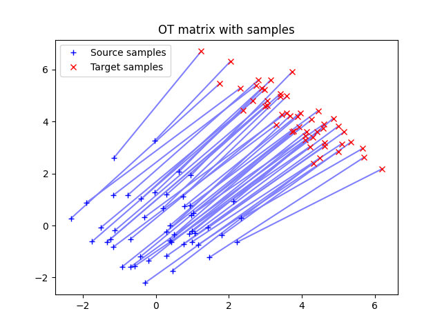
Optional: optimal transport

One strategy to assign images to pixels is to search the image that matches the color of the pixel the closest. You will get a lot of the same images though. The cooler challenge is to do the assignment such that every cat picture is only used once!

It turns out that this is one of the hardest problems in computer science and is known by many names. Though not all identical, all these problems are related:

• Monge’s (Ampère and Kantorovich can also be found in naming this) problem: suppose you have a number of mines in several places, and refineries in other places. You want to move ore to all the refineries in such a way that the total mass transport is minimized.
• Stable Mariage problem: suppose you have $n$ men and $n$ women (all straight, this problem was first stated somewhere in the 1950ies) and want to create $n$ couples, such that no man desires another’s wife that also desires that man over her own spouse.
• Optimal Mariage problem: in the previous setting can you find the solution that makes everyone the happiest globally?
• Find the least “costly” mapping from one probability distribution to another.

These problems generally belong to the topic of optimal transport. There is a nice Python library, Python Optimal Transport, or pot for short, that implements many algorithms for solving optimal transport problems. Check out the POT Documentation.

Solution

This code is adapted from an example on the OT documentation. Suppose that you have two arrays of sizes (m, 3) and (n, 3), where n is the amount of cat pictures, and m the amount of pixels in the target. Each array lists the RGB values that you want to match, thumbs_rgb and target_rgb.

import ot

n = len(thumbs_rgb)
m = len(target_rgb)
M = ot.dist(thumbs_rgb, target_rgb)
M /= M.max()
G0 = ot.emd(np.ones((n,))/n, np.ones((m,))/m, M, numItermax=10**6)

matches = np.argmax(G0, axis=0)
print("Unique images used in optimal transport approach: {}" \
      .format(np.unique(matches).shape[0]))
np.savetxt(
    data_path / "matches_unique.tab",
    matches.reshape(target_res),
    fmt="%d")

Key Points

• You sometimes have to try different strategies to find out what works best.

Exercise: Mandelbrot fractals

Overview

Teaching: 15 min
Exercises: 75 min

Questions

• How do I decide which technique to use where?

• How do I put everything together?

• Can you show some real life examples?

Objectives

• Create a strategy for parallelising existing code.

• Apply previously discussed methods to problems.

• Choose the correct abstraction for a problem.

The Mandelbrot and Julia fractals

This exercise uses Numpy and Matplotlib.

from matplotlib import pyplot as plt
import numpy as np

We will be computing the famous Mandelbrot fractal. The Mandelbrot set is the set of complex numbers \(c \in \mathbb{C}\) for which the iteration,

[z_{n+1} = z_n^2 + c,]

converges, starting iteration at \(z_0 = 0\). We can visualize the Mandelbrot set by plotting the number of iterations needed for the absolute value \(|z_n|\) to exceed 2 (for which it can be shown that the iteration always diverges).

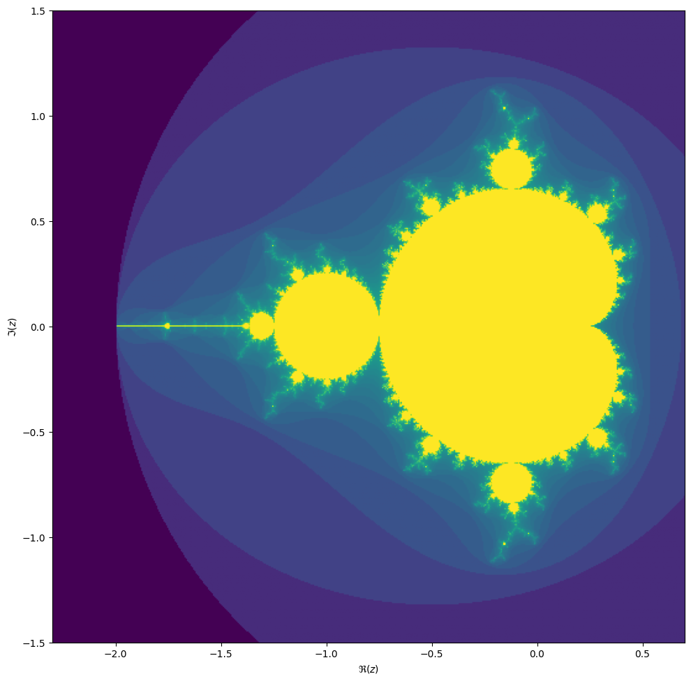
We may compute the Mandelbrot as follows:

max_iter = 256
width = 256
height = 256
center = -0.8+0.0j
extent = 3.0+3.0j
scale = max((extent / width).real, (extent / height).imag)

result = np.zeros((height, width), int)
for j in range(height):
    for i in range(width):
        c = center + (i - width // 2 + (j - height // 2)*1j) * scale
        z = 0
        for k in range(max_iter):
            z = z**2 + c
            if (z * z.conjugate()).real > 4.0:
                break
        result[j, i] = k

Then we can plot with the following code:

fig, ax = plt.subplots(1, 1, figsize=(10, 10))
plot_extent = (width + 1j * height) * scale
z1 = center - plot_extent / 2
z2 = z1 + plot_extent
ax.imshow(result**(1/3), origin='lower', extent=(z1.real, z2.real, z1.imag, z2.imag))
ax.set_xlabel("$\Re(c)$")
ax.set_ylabel("$\Im(c)$")

Things become really loads of fun when we start to zoom in. We can play around with the center and extent values (and necessarily max_iter) to control our window.

max_iter = 1024
center = -1.1195+0.2718j
extent = 0.005+0.005j

When we zoom in on the Mandelbrot fractal, we get smaller copies of the larger set!

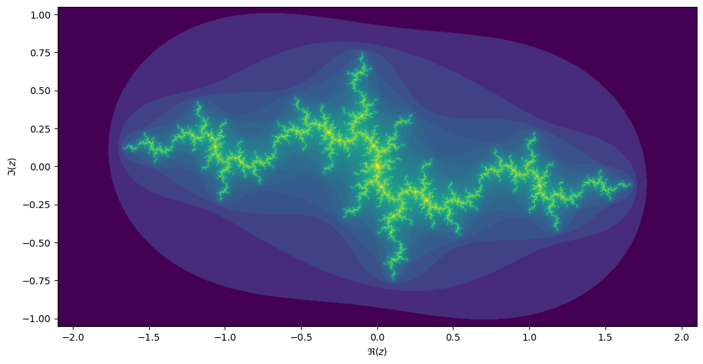
Julia sets

For each value \(c\) we can compute the Julia set, namely the set of starting values \(z_1\) for which the iteration over \(z_{n+1}=z_n^2 + c\) converges. Every location on the Mandelbrot image corresponds to its own unique Julia set.

max_iter = 256
center = 0.0+0.0j
extent = 4.0+3.0j
scale = max((extent / width).real, (extent / height).imag)

result = np.zeros((height, width), int)
c = -1.1193+0.2718j

for j in range(height):
    for i in range(width):
        z = center + (i - width // 2 + (j - height // 2)*1j) * scale
        for k in range(max_iter):
            z = z**2 + c
            if (z * z.conjugate()).real > 4.0:
                break
        result[j, i] = k

If we take the center of the last image, we get the following rendering of the Julia set:

Exercise

Make this into a parallel program. What kind of speed-ups do you get? Can you get it efficient enough so that your code could power an interactive fractal zoomer?

Hint: to structure the code, you may want to create a GridInfo class:

from dataclasses import dataclass
from typing import Callable
import numpy as np

@dataclass
class GridInfo:
    width: int
    height: int
    center: complex
    extent: complex

    def map_int(f, *args):
         """Compute the value of `f(z)` for every point in this
         grid-info object. You may pass extra arguments to `f` as
         extra arguments to this function.

         Returns: np.ndarray of size (width, height)"""
         ...

Then you may specify the function for computing the Mandelbrot fractal:

def iteration_count(f, stop: Callable[(complex,), bool],
                    start: complex, max_iter: int, *args) -> int:
    x = start
    for k in range(max_iter):
        x = f(x, *args)
        if stop(x):
            break
    return k

def stop_condition(z: complex):
    return (z.conj() * z).real > 4.0

def mandelbrot(max_iter: int):
    def mandelbrot_f(c: complex):
        return iteration_count(lambda z: z**2 + c, stop_condition, 0, max_iter)
    return mandelbrot_f

These functions can be JIT compiled with Numba.

Optional

There is another way to compute the Julia fractal: inverse iteration method (IIM). Here you are computing the inverse of \(z_{n} = z_{n-1}^2 + c\),

\[z_{n-1} = \sqrt{z_n - c}.\]

Because this inverse is multi-valued, your set of points grows exponentially with each inverse iteration. This can be solved by randomly selecting a path at each iteration.

Optional

See if you can make your solution work with the following ipywidgets code. You may have to restructure either your own code or this snippet, whichever you prefer.

You need ipympl installed, for this to work.

conda install -c conda-forge ipympl
conda install -c conda-forge nodejs
jupyter labextension install @jupyter-widgets/jupyterlab-manager jupyter-matplotlib
# restart Jupyter

%matplotlib widget
import ipywidgets as widgets

fig, ax = plt.subplots(1, 2, figsize=(10, 5))

# Plot the Mandelbrot to ax[0]; for this to work you need
# a function `plot_fractal` that plots the fractal for you,
# and a precomputed mandelbrot in `mandelbrot_im`.
mandel_grid = GridInfo(256, 256, -0.8+0.0j, 3.0+2.0j)
mandelbrot_im = mandel_grid.int_map(mandelbrot(256))
plot_fractal(mandel_grid, np.log(mandelbrot_im+1), ax=ax[0])

# Add a marker for the selector location
mbloc = ax[0].plot(0, 0, 'r+')

# This function only updates the position of the marker
def update_mandel_plot(c):
    mbloc[0].set_xdata(c.real)
    mbloc[0].set_ydata(c.imag)
    fig.canvas.draw()

# `julia_ic` should return a Numba optimized function that
# iterates `z = z^2 + c` for a `c` that is given as an extra
# parameter.
julia_fun = julia(256)
julia_grid = GridInfo(256, 256, 0.0+0.0j, 3+3j)
julia_im = julia_grid.int_map(julia_fun, 0)
plot_fractal(julia_grid, np.log(julia_im + 1), ax=ax[1])

def update_julia_plot(c):
    julia_im = julia_grid.int_map(julia_it, c)
    plot_fractal(julia_grid, np.log(julia_im + 1), ax=ax[1])

@widgets.interact(x=(-2, 1.0, 0.01), y=(-1.5, 1.5, 0.01))
def update(x, y):
    c = x + 1j * y
    update_mandel_plot(c)
    update_julia_plot(c)

plt.tight_layout()

Key Points

• You sometimes have to try different strategies to find out what works best.

Dynamic programming

Overview

Teaching: 0 min
Exercises: 0 min

Questions

• How can I save intermediate result and recover from crashes?

• How can I prevent duplicate computations?

Objectives

• Understand the principles of dynamic programming.

• Understand the relevance of dynamic programming in a parallel environment.

• Write a parallel sudoku solver

FIXME

Key Points

• FIXME

Calling external C and C++ libraries from Python

Overview

Teaching: 60 min
Exercises: 30 min

Questions

• What are some of my options in calling C and C++ libraries from Python code?

• How does this work together with Numpy arrays?

• How do I use this in multiple threads while lifting the GIL?

Objectives

• Compile and link simple C programs into shared libraries.

• Call these library from Python and time its executions.

• Compare the performance with Numba decorated Python code.

• Bypass the GIL when calling these libraries from multiple threads simultaneously.

Calling C and C++ libraries

Simple example using either pybind11 or ctypes

External C and C++ libraries can be called from Python code using a number of options, using e.g. Cython, CFFI, pybind11 and ctypes. We will discuss the last two, because they require the least amount of boilerplate, for simple cases - for more complex examples that may not be the case. Consider this simple C program, test.c, which adds up consecutive numbers:

#include <pybind11/pybind11.h>
namespace py = pybind11;

long long sum_range(long long high)
{
  long long i;
  long long s = 0LL;

  for (i = 0LL; i < high; i++)
      s += (long long)i;

  return s;
}

PYBIND11_MODULE(test_pybind, m) {
    m.doc() = "Export the sum_range function as sum_range";

    m.def("sum_range", &sum_range, "Adds upp consecutive integer numbers from 0 up to and including high-1");
}

You can easily compile and link it into a shared object (.so) file. First you need pybind11. You can install it in a number of ways, like pip, but I prefer creating virtual environments using pipenv.

pip install pipenv
pipenv install pybind11
pipenv shell

c++ -O3 -Wall -shared -std=c++11 -fPIC `python3 -m pybind11 --includes` test.c -o test_pybind.so

which generates a test_pybind.so shared object which you can call from a iPython shell, like this:

%import test_pybind
%sum_range=test_pybind.sum_range
%high=1000000000
%brute_force_sum=sum_range(high)

Now you might want to check the output, by comparing with the well-known formula for the sum of consecutive integers.

%sum_from_formula=high*(high-1)//2
%sum_from_formula
%difference=sum_from_formula-brute_force_sum
%difference

Give this script a suitable name, like call_C_libraries.py. The same thing can be done using ctypes instead of pybind11, but requires slightly more boilerplate on the Python side of the code and slightly less on the C side. test.c will be just the algorithm:

long long sum_range(long long high)
{
  long long i;
  long long s = 0LL;

  for (i = 0LL; i < high; i++)
      s += (long long)i;

  return s;
}

Compile and link using

gcc -O3 -g -fPIC -c -o test.o test.c
ld -shared -o libtest.so test.o

which generates a libtest.so file.

You will need some extra boilerplate:

%import ctypes
%testlib = ctypes.cdll.LoadLibrary("./libtest.so")
%sum_range = testlib.sum_range
%sum_range.argtypes = [ctypes.c_longlong]
%sum_range.restype = ctypes.c_longlong
%high=1000000000
%brute_force_sum=sum_range(high)

Again, you can compare with the formula for the sum of consecutive integers.

%sum_from_formula=high*(high-1)/2
%sum_from_formula
%difference=sum_from_formula-brute_force_sum
%difference

Performance

Now we can time our compiled sum_range C library, e.g. from the iPython interface:

%timeit sum_range(10**7)

2.69 ms ± 6.01 µs per loop (mean ± std. dev. of 7 runs, 100 loops each)

If you compare with the Numba timing from chapter 3, you will see that the C library for sum_range is faster than the numpy computation but significantly slower than the numba.jit decorated function.

Challenge: Check if the Numba version of this conditional sum range function outperforms its C counterpart:

Insprired by a blog by Christopher Swenson.

long long conditional_sum_range(long long to)
{
  long long i;
  long long s = 0LL;

  for (i = 0LL; i < to; i++)
    if (i % 3 == 0)
      s += i;

  return s;
}

Solution

Just insert a line if i%3==0: in the code for sum_range_numba and rename it to conditional_sum_range_numba.

@numba.jit
def conditional_sum_range_numba(a: int):
    x = 0
    for i in range(a):
        if i%3==0:
            x += i
    return x

Let’s check how fast it runs.

%timeit conditional_sum_range_numba(10**7)

8.11 ms ± 15.6 µs per loop (mean ± std. dev. of 7 runs, 100 loops each)

Compare this with the run time for the C code for conditional_sum_range. Compile and link in the usual way, assuming the file name is still test.c:

gcc -O3 -g -fPIC -c -o test.o test.c
ld -shared -o libtest.so test.o

Again, we can time our compiled conditional_sum_range C library, e.g. from the iPython interface:

import ctypes
testlib = ctypes.cdll.LoadLibrary("./libtest.so")
conditional_sum_range = testlib.conditional_sum_range
conditional_sum_range.argtypes = [ctypes.c_longlong]
conditional_sum_range.restype = ctypes.c_longlong
%timeit conditional_sum_range(10**7)

7.62 ms ± 49.7 µs per loop (mean ± std. dev. of 7 runs, 100 loops each)

This shows that for this slightly more complicated example the C code is somewhat faster than the Numba decorated Python code.

Passing Numpy arrays to C libraries.

Now let us consider a more complex example. Instead of computing the sum of numbers up to a certain upper limit, let us compute that for an array of upper limits. This will return an array of sums. How difficult is it to modify our C and Python code to get this done? Well, you just need to replace &sum_range by py::vectorize(sum_range):

PYBIND11_MODULE(test_pybind, m) {
    m.doc() = "pybind11 example plugin"; // optional module docstring

    m.def("sum_range", py::vectorize(sum_range), "Adds upp consecutive integer numbers from 0 up to and including high-1");
}

Now let’s see what happens if we pass test_pybind.so an array instead of an integer.

%import test_pybind
%sum_range=test_pybind.sum_range
%ys=range(10)
%sum_range(ys)

gives

array([ 0,  0,  1,  3,  6, 10, 15, 21, 28, 36])

It does not crash! Instead, it returns an array which you can check to be correct by subtracting the previous sum from each sum (except the first):

%out=sum_range(ys)
%out[1:]-out[:-1]

which gives

array([0, 1, 2, 3, 4, 5, 6, 7, 8])

the elements of ys - except the last - as you would expect.

Call the C library from multiple threads simultaneously.

We can quickly show you how the C library compiled using pybind11 can be run multithreaded. try the following from an iPython shell:

%high=int(1e9)
%timeit(sum_range(high))

gives

274 ms ± 1.03 ms per loop (mean ± std. dev. of 7 runs, 1 loop each)

Now try a straightforward parallellisation of 20 calls of sum_range, over two threads, so 10 calls per thread. This should take about 10 * 274ms = 2.74s if parallellisation were running without overhead. Let’s try:

%import threading as T
%import time
%def timer():
%    start_time = time.time()
%    for x in range(10):
%        t1 = T.Thread(target=sum_range, args=(high,))
%        t2 = T.Thread(target=sum_range, args=(high,))
%        t1.start()
%        t2.start()
%        t1.join()
%        t2.join()
%    end_time = time.time()
%    print(f"Time elapsed = {end_time-start_time:.2f}s")
%timer()

This gives

Time elapsed = 5.59s

i.e. more than twice the time we would expect. What actually happened is that sum_range was run sequentially instead of parallelly. We need to add a single declaration to test.c: py::call_guard<py::gil_scoped_release>():

PYBIND11_MODULE(test_pybind, m) {
    m.doc() = "pybind11 example plugin"; // optional module docstring

    m.def("sum_range", py::vectorize(sum_range), "Adds upp consecutive integer numbers from 0 up to and including high-1");
}

like this:

PYBIND11_MODULE(test_pybind, m) {
    m.doc() = "pybind11 example plugin"; // optional module docstring

    m.def("sum_range", &sum_range, "A function which adds upp numbers from 0 up to and including high-1", py::call_guard<py::gil_scoped_release>());
}

Now compile again:

c++ -O3 -Wall -shared -std=c++11 -fPIC `python3 -m pybind11 --includes` test.c -o test_pybind.so

Reimport the rebuilt shared object - this can only be done by quitting and relaunching the iPython interpreter - and time again.

%import test_pybind
%import time
%import threading as T
%
%sum_range=test_pybind.sum_range
%high=int(1e9)
%
%def timer():
%    start_time = time.time()
%    for x in range(10):
%        t1 = T.Thread(target=sum_range, args=(high,))
%        t2 = T.Thread(target=sum_range, args=(high,))
%        t1.start()
%        t2.start()
%        t1.join()
%        t2.join()
%    end_time = time.time()
%    print(f"Time elapsed = {end_time-start_time:.2f}s")
%timer()

This gives:

Time elapsed = 2.81s

as you would expect for two sum_range modules running in parallel.

Key Points

• Multiple options are available in calling external C and C++ libraries and that the best choice can depend on the complexity of your problem.

• Obviously, there is an extra compile and link step, but you will get a much faster execution compared to pure Python.

• Also, the GIL will be circumvented in calling these libaries.

• Numba might also offer you the speedup you want with even less effort.

Asyncio fundamentals

Overview

Teaching: 40 min
Exercises: 20 min

Questions

• What is AsyncIO?

• How do I structure an async program?

Objectives

• Understand the different mental model of asynchronous program execution flow.

• Understand the difference between a function and a coroutine.

• Create classic generators, use the yield keyword.

• Setup an async program with an event loop using asyncio.run().

• Create an asynchronous generator, use async and await keywords.

Asyncio

This is not for everyone. You may encounter asyncio in the wild though.

Different runtime

With functions (FIXME: make a graphic):

  call f
  |      ---> new context: f
  |           | do work
  |      <--- | return result (context destroyed)
  | use result

With generators (FIXME: make a graphic):

  call f
  |               ---> new context: f
  |               <--- | yield
  | do some work
  | ask f         ---> | continue in old context
  |                    | do some work
  |               <--- | yield result
  | work with result
  | ask f again   ---> | do some more work
  |               <--- | yield another result
  | yay!

A coroutine returns to its previous state on the next call. Let’s see an example. We compute the Fibonacci numbers:

def fib():
  a, b = 1, 1
  while True:
    yield a
    a, b = b, a + b

To see if this is working

from itertools import islice
list(islice(fib(), 20))

We can run the generator step by step:

x = fib()
for i in range(20):
  n = next(x)
  print(f"{i:8} {n:8}")

It is possible to model light weight threading using generators. On the background there is a event loop that manages a set of coroutines. Each coroutine is entered similar to a normal generator and gives back control to the event loop through await, similar to yield (actually await is synonymous to yield from).

import asyncio

async def fun_a():
    print("Running coroutine *a*.")
    await asyncio.sleep(0)
    print("Back in *a*.")
    return "result from *a*"

async def fun_b():
    print("Running coroutine *b*.")
    await asyncio.sleep(0)
    print("Back in *b*.")
    return "result from *b*"

await asyncio.gather(fun_a(), fun_b())

Event loop

It is important to have an event-loop running before you do anything else:

import asyncio

async def main()
    # Initialize any Task, Lock or Semaphore inside main()
    await work

asyncio.run(main())

However, Jupyter already runs in an async loop, so we should just:

await main()

##

Key Points

• Programs are parallelizable if you can identify independent tasks.