Overview

Teaching: 15 min
Exercises: 75 min

Questions

• How do I decide which technique to use where?

• How do I put everything together?

• Can you show some real life examples?

Objectives

• Create a strategy for parallelising existing code.

• Apply previously discussed methods to problems.

• Choose the correct abstraction for a problem.

The Mandelbrot and Julia fractals

This exercise uses Numpy and Matplotlib.

from matplotlib import pyplot as plt
import numpy as np

We will be computing the famous Mandelbrot fractal. The Mandelbrot set is the set of complex numbers \(c \in \mathbb{C}\) for which the iteration,

converges, starting iteration at \(z_0 = 0\). We can visualize the Mandelbrot set by plotting the number of iterations needed for the absolute value \(|z_n|\) to exceed 2 (for which it can be shown that the iteration always diverges).

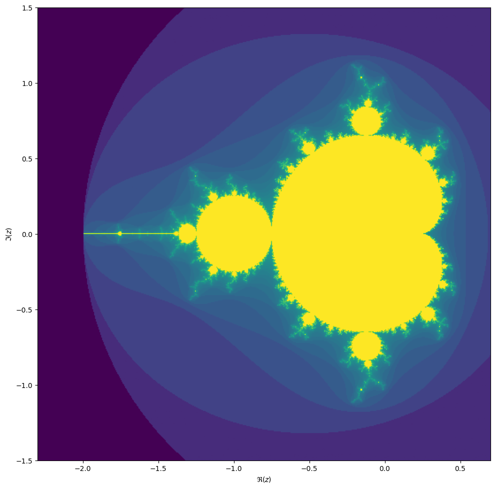
We may compute the Mandelbrot as follows:

max_iter = 256
width = 256
height = 256
center = -0.8+0.0j
extent = 3.0+3.0j
scale = max((extent / width).real, (extent / height).imag)

result = np.zeros((height, width), int)
for j in range(height):
    for i in range(width):
        c = center + (i - width // 2 + (j - height // 2)*1j) * scale
        z = 0
        for k in range(max_iter):
            z = z**2 + c
            if (z * z.conjugate()).real > 4.0:
                break
        result[j, i] = k

Then we can plot with the following code:

fig, ax = plt.subplots(1, 1, figsize=(10, 10))
plot_extent = (width + 1j * height) * scale
z1 = center - plot_extent / 2
z2 = z1 + plot_extent
ax.imshow(result**(1/3), origin='lower', extent=(z1.real, z2.real, z1.imag, z2.imag))
ax.set_xlabel("$\Re(c)$")
ax.set_ylabel("$\Im(c)$")

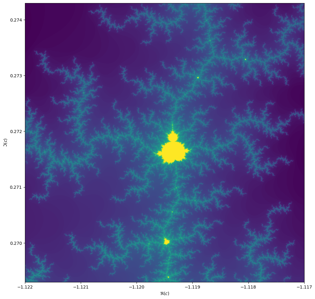
Things become really loads of fun when we start to zoom in. We can play around with the center and extent values (and necessarily max_iter) to control our window.

max_iter = 1024
center = -1.1195+0.2718j
extent = 0.005+0.005j

When we zoom in on the Mandelbrot fractal, we get smaller copies of the larger set!

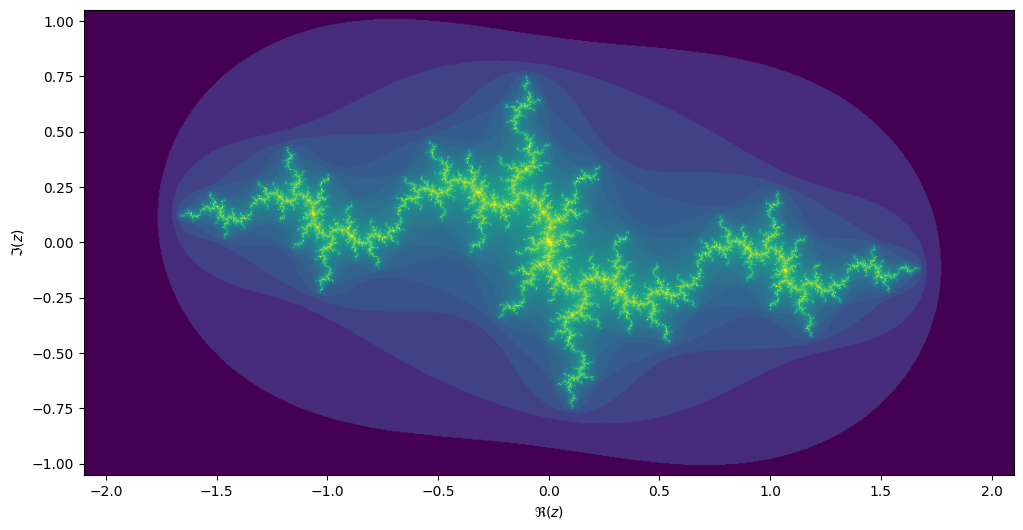
Julia sets

For each value \(c\) we can compute the Julia set, namely the set of starting values \(z_1\) for which the iteration over \(z_{n+1}=z_n^2 + c\) converges. Every location on the Mandelbrot image corresponds to its own unique Julia set.

max_iter = 256
center = 0.0+0.0j
extent = 4.0+3.0j
scale = max((extent / width).real, (extent / height).imag)

result = np.zeros((height, width), int)
c = -1.1193+0.2718j

for j in range(height):
    for i in range(width):
        z = center + (i - width // 2 + (j - height // 2)*1j) * scale
        for k in range(max_iter):
            z = z**2 + c
            if (z * z.conjugate()).real > 4.0:
                break
        result[j, i] = k

If we take the center of the last image, we get the following rendering of the Julia set:

Exercise

Make this into a parallel program. What kind of speed-ups do you get? Can you get it efficient enough so that your code could power an interactive fractal zoomer?

Hint: to structure the code, you may want to create a GridInfo class:

from dataclasses import dataclass
from typing import Callable
import numpy as np

@dataclass
class GridInfo:
    width: int
    height: int
    center: complex
    extent: complex

    def map_int(f, *args):
         """Compute the value of `f(z)` for every point in this
         grid-info object. You may pass extra arguments to `f` as
         extra arguments to this function.

         Returns: np.ndarray of size (width, height)"""
         ...

Then you may specify the function for computing the Mandelbrot fractal:

def iteration_count(f, stop: Callable[(complex,), bool],
                    start: complex, max_iter: int, *args) -> int:
    x = start
    for k in range(max_iter):
        x = f(x, *args)
        if stop(x):
            break
    return k

def stop_condition(z: complex):
    return (z.conj() * z).real > 4.0

def mandelbrot(max_iter: int):
    def mandelbrot_f(c: complex):
        return iteration_count(lambda z: z**2 + c, stop_condition, 0, max_iter)
    return mandelbrot_f

These functions can be JIT compiled with Numba.

Optional

There is another way to compute the Julia fractal: inverse iteration method (IIM). Here you are computing the inverse of \(z_{n} = z_{n-1}^2 + c\),

\[z_{n-1} = \sqrt{z_n - c}.\]

Because this inverse is multi-valued, your set of points grows exponentially with each inverse iteration. This can be solved by randomly selecting a path at each iteration.

Optional

See if you can make your solution work with the following ipywidgets code. You may have to restructure either your own code or this snippet, whichever you prefer.

You need ipympl installed, for this to work.

conda install -c conda-forge ipympl
conda install -c conda-forge nodejs
jupyter labextension install @jupyter-widgets/jupyterlab-manager jupyter-matplotlib
# restart Jupyter

%matplotlib widget
import ipywidgets as widgets

fig, ax = plt.subplots(1, 2, figsize=(10, 5))

# Plot the Mandelbrot to ax[0]; for this to work you need
# a function `plot_fractal` that plots the fractal for you,
# and a precomputed mandelbrot in `mandelbrot_im`.
mandel_grid = GridInfo(256, 256, -0.8+0.0j, 3.0+2.0j)
mandelbrot_im = mandel_grid.int_map(mandelbrot(256))
plot_fractal(mandel_grid, np.log(mandelbrot_im+1), ax=ax[0])

# Add a marker for the selector location
mbloc = ax[0].plot(0, 0, 'r+')

# This function only updates the position of the marker
def update_mandel_plot(c):
    mbloc[0].set_xdata(c.real)
    mbloc[0].set_ydata(c.imag)
    fig.canvas.draw()

# `julia_ic` should return a Numba optimized function that
# iterates `z = z^2 + c` for a `c` that is given as an extra
# parameter.
julia_fun = julia(256)
julia_grid = GridInfo(256, 256, 0.0+0.0j, 3+3j)
julia_im = julia_grid.int_map(julia_fun, 0)
plot_fractal(julia_grid, np.log(julia_im + 1), ax=ax[1])

def update_julia_plot(c):
    julia_im = julia_grid.int_map(julia_it, c)
    plot_fractal(julia_grid, np.log(julia_im + 1), ax=ax[1])

@widgets.interact(x=(-2, 1.0, 0.01), y=(-1.5, 1.5, 0.01))
def update(x, y):
    c = x + 1j * y
    update_mandel_plot(c)
    update_julia_plot(c)

plt.tight_layout()

Key Points

• You sometimes have to try different strategies to find out what works best.