BGC Similarity Networks

Overview

Teaching: 30 min
Exercises: 15 min

Questions

• How can I measure similarity between BGCs?

Objectives

• Understand how BiG-SCAPE measures similarity between BGCs.

• Take an antiSMASH output to perform a BiG-SCAPE analysis.

• Interpret BiG-SCAPE similarity networks and GCF phylogenies.

Introduction

In the previous section, we learned how to study the BGCs encoded by each of the genomes of our analyses. In case you are interested in the study of a certain BGC or a certain strain, this may be enough. However, sometimes the aim is to compare the biosynthetic potential of tens or hundreds of genomes. To perform this kind of analysis, we will use BiG-SCAPE (Navarro-Muñoz et al., 2019), a workflow that compares all the BGCs detected by antiSMASH to find their relatedness. BiG-SCAPE will search for Pfam domains (Mistry et al., 2021) in the protein sequences of each BGC. Then, the Pfam domains will be linearized and compared, creating different similarity networks and scoring the similarity of each pair of clusters. Based on a cutoff value for this score, the diverse BGCs will be classified on Gene Cluster Families (GCFs) to facilitate their study. A single GCF is supposed to encompass BGCs that produce chemically related metabolites (molecular families). Lower cutoffs would create families of BGCs that produce identical compounds, while higher cutoffs would create families of more loosely related compounds.

Preparing the input

In each of the antiSMASH output directories, we will find a single .gbk file for each BGC, which includes “region” within its filename. Thus, we will copy all these files to the new directory.

Move into the directory that has the antiSMASH results of each genome:

$ conda deactivate  
$ conda activate /miniconda3/envs/bigscape/  
$ cd ~/pan_workshop/results/antismash/
$ ls

Since we will put together in the same directory many files with similar names, we want to make sure that nothing is left behind or overwritten. For this, we will count all the gbk files of all the genomes.

$ ls Streptococcus_agalactiae_*/*region*gbk | wc -l

16

Since the names are somewhat cryptic, they could be repeated, so we will rename the gbks in such a way that they include the genome name.

Copy the following script to a file named change-names.sh using nano:

# This script is to rename the antiSMASH gbks for them to include the species and strain names, taken from the directory name.
# The argument it requires is the name of the directory with the AntiSMASH output, which must NOT contain a slash at the end.

# Usage for one AntiSMASH output directory:
#     sh change-names.sh <folder>

# Usage for multiple AntiSMASH output directory:
#     for species in <output-directory-pattern*>
#    	 do
#    		 sh change-names.sh $species
#    	 done



ls -1 "$1"/*region*gbk | while read line # enlist the gbks of all regions in the directory and start a while loop
 do
    dir=$(echo $line | cut -d'/' -f1) # save the directory name in a variable
    file=$(echo $line | cut -d'/' -f2) # save the file name in a variable
	for directory in $dir # start a for loop
    	do
   		 cd $directory # enter the directory
      	newfile=$(echo $dir-$file) # make a new variable that fuses the directory name with the file name
			 	echo "Renaming" $file " to" $newfile # print a message showing the old and new file names
			 	mv $file $newfile # rename
			 	cd .. # return to main directory before it begins again
		 done
 done

Run the script for all the directory:

$ for species in Streptococcus_agalactiae_*
> do
>   	 sh change-names.sh $species
>    done

Now make a directory for all your BiG-SCAPE analyses and inside it make a directory that contains all of the gbks of all of your genomes. This one will be the input for BiG-SCAPE. (For convenience bigscape/ will be inside antismash/ while we run BiG-SCAPE).

$ mkdir -p bigscape/bgcs_gbks/

Now copy all the region gbksto this new directory, and look at its content:

$ cp Streptococcus_agalactiae_*/*region*gbk bigscape/bgcs_gbks/
$ ls bigscape/bgcs_gbks/

Streptococcus_agalactiae_18RS21_prokka-AAJO01000016.1.region001.gbk
Streptococcus_agalactiae_18RS21_prokka-AAJO01000043.1.region001.gbk
Streptococcus_agalactiae_2603V_prokka-NC_004116.1.region001.gbk
Streptococcus_agalactiae_2603V_prokka-NC_004116.1.region002.gbk
Streptococcus_agalactiae_515_prokka-NZ_CP051004.1.region001.gbk
Streptococcus_agalactiae_515_prokka-NZ_CP051004.1.region002.gbk
Streptococcus_agalactiae_A909_prokka-NC_007432.1.region001.gbk
Streptococcus_agalactiae_A909_prokka-NC_007432.1.region002.gbk
Streptococcus_agalactiae_CJB111_prokka-NZ_AAJQ01000010.region001.gbk
Streptococcus_agalactiae_CJB111_prokka-NZ_AAJQ01000025.region001.gbk
Streptococcus_agalactiae_COH1_prokka-NZ_HG939456.1.region001.gbk
Streptococcus_agalactiae_COH1_prokka-NZ_HG939456.1.region002.gbk
Streptococcus_agalactiae_H36B_prokka-AAJS01000020.1.region001.gbk
Streptococcus_agalactiae_H36B_prokka-AAJS01000117.1.region001.gbk
Streptococcus_agalactiae_NEM316_prokka-NC_004368.1.region001.gbk
Streptococcus_agalactiae_NEM316_prokka-NC_004368.1.region002.gbk

Running BiG-SCAPE

BiG-SCAPE can be executed in different ways, depending on the installation mode that you applied. You could call the program through bigscape, run_bigscapeor run_bigscape.py. Here, based on our installation (see Setup), we will use run_bigscape.

The options that we will use are described in the help page:

-i INPUTDIR, --inputdir INPUTDIR
                    	Input directory of gbk files, if left empty, all gbk
                    	files in current and lower directories will be used.

-o OUTPUTDIR, --outputdir OUTPUTDIR
                    	Output directory, this will contain all output data
                    	files.

--mix             	By default, BiG-SCAPE separates the analysis according
                   	to the BGC product (PKS Type I, NRPS, RiPPs, etc.) and
                   	will create network directories for each class. Toggle
                   	to include an analysis mixing all classes
                  	 
--hybrids-off     	Toggle to also add BGCs with hybrid predicted products
                    	from the PKS/NRPS Hybrids and Others classes to each
                    	subclass (e.g. a 'terpene-nrps' BGC from Others would
                    	be added to the Terpene and NRPS classes)

--mode {global,glocal,auto}
                    	Alignment mode for each pair of gene clusters.
                    	'global': the whole list of domains of each BGC are
                    	compared; 'glocal': Longest Common Subcluster mode.
                    	Redefine the subset of the domains used to calculate
                    	distance by trying to find the longest slice of common
                    	domain content per gene in both BGCs, then expand each
                    	slice. 'auto': use glocal when at least one of the
                    	BGCs in each pair has the 'contig_edge' annotation
                    	from antiSMASH v4+, otherwise use global mode on that
                    	pair

We will use the option --mix to have an analysis of all of the BGCs together besides the analyses of the BGCs separated by class. The --hybrids-off option will prevent from having the same BGC twice (in the case of hybrid BGCs that could belong to two classes) in our results. And since none of the BGCs is on a contig edge, we could use the global mode. However, frequently, when analyzing draft genomes, this is not the case. Thus, the auto mode will be the most appropriate, which will use the global mode to align domains except for those cases in which the BGC is located near to a contig end, for which the glocal mode is automatically selected. For this run we will use only the default cutoff value (0.3).

Now we are ready to run BiG-SCAPE:

$ bigscape -i bigscape/bgcs_gbks/ -o bigscape/output_220124 --mix --hybrids-off --mode auto --pfam_dir /miniconda3/envs/bigscape/BiG-SCAPE-1.1.5/

Output names

Most of the times you will need to re-run a software once you have explored the results; maybe you want to change parameters or add more samples. For this reason, you will need a flexible way to organize your project, including the names of the outputs. Usually, a good idea is to put the date in the name of the folder and keep track of the analyses you are running in your research notes.

Once the process is finished, you will find in your terminal screen some basic results, such as the number of BGCs included in each type of network. In the output folder you will find all the data.
Since BiG-SCAPE does not produce a file with the run information, it is useful to copy the text printed on the screen to a file. Use nano to paste all the text that BiG-SCAPE generated in a file named bigscape.log inside the folder output_100722/logs/.

$ nano bigscape/output_220124/logs/bigscape.log

Take a look at the BiG-SCAPE outputs:

$ ls -F bigscape/output_220124/

cache/  html_content/  index.html*  logs/  network_files/  SVG/

To keep ordered your directories, move your bigscape/ directory to results/:

$ mv bigscape/ ../

And move the file change-names to folder scripts/ in the pan_workshop/directory to save our little script:

$ mv change-names.sh ~/pan_workshop/scripts/

Viewing the results

An easy way to prospect your results is by opening the index.html file with a browser (Firefox, Chrome, Safari, etc.). In order to do this, you need to go to your local machine and locate in the folder where you want to store your BiG-SCAPE results. Now we compress the folder output_100622/ and download it to your local machine.

$ cd ~/pan_workshop/results/bigscape/
$ zip -r output_220124.zip output_220124
$ ls

In the JupyterHub we navigate to the folders and go to /pan_workshop/results/bigscape and select the one we just created output_220124.zip and download it.

On your local computer we unzip the files and open output_220124/index.html with a browser:

$ firefox output_100622/index.html # If you have Firefox available, otherwise open it using the GUI.

There are diverse sections in the visualization. The following image shows the overview page. At the left there is the run information and there are pie chart representations of the number of BGCs per genome and per class. At the right there is the Network Overview for each of the BGC classes found and the mix category. They show the Number of Families, Average number of BGCs per family, Max number of BGCs in a family and the Families with MIBiG Reference BGCs. You can click on the name of the class to see its Network Overview.

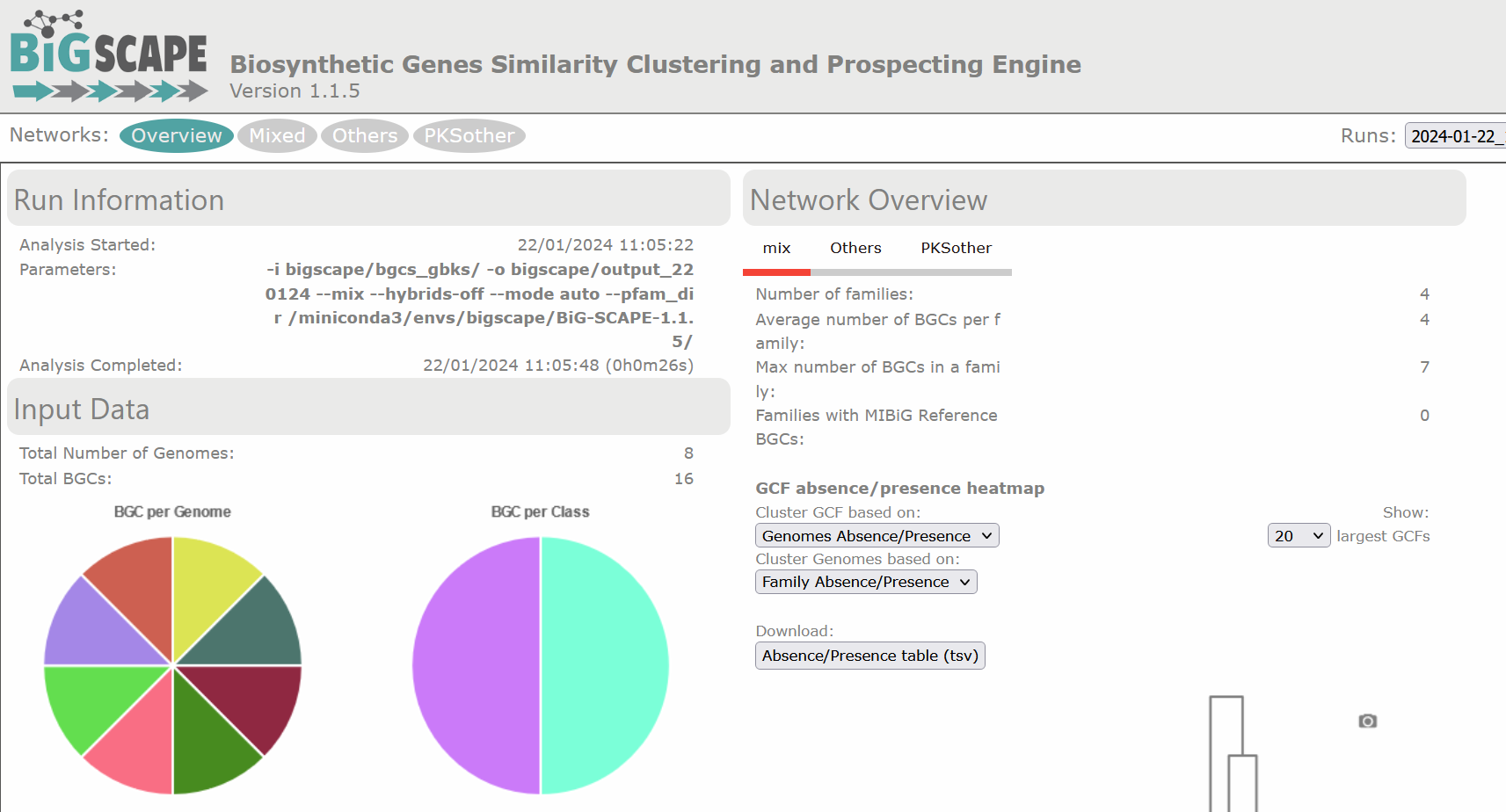
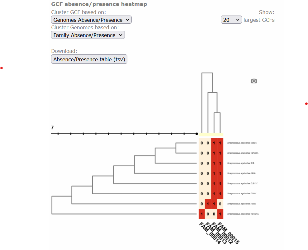
Below, there is a clustered heatmap of the presence/absence of the GCFs in each genome for each class. You can customize this heatmap and select the clustering methods, or the number of GCFs represented.

Clicking any of the class names of the upper left bar displays a similarity network of BGCs. It may take some time to load the network. A single network is represented for each GCF of each Gene Cluster Clan (GCC), which may comprise several GCFs. Each dot represents a BGC. These dots with bold circles are already described BGCs that have been recruited from the MiBIG database (Kautsar et al., 2020) because of its similarity with some BGC of the analysis.

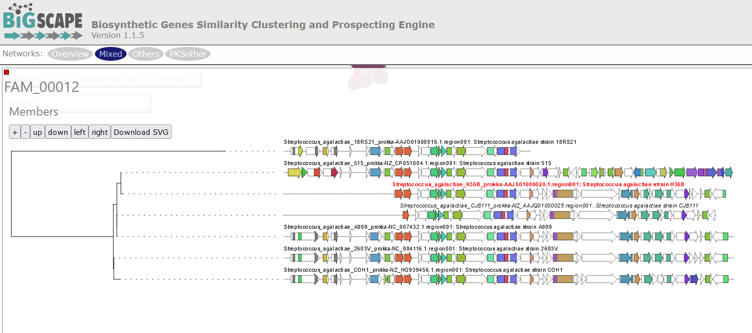
When you click on a BGC (dot), it appears its GCF at the right. You can click on the GCF name to see the phylogenetic distances among all the BGCs comprised by a single GCF. Within the tree there is an arrow diagram of the genes in the BGCs and the protein domains in the genes. These trees are useful to prioritize the search of secondary metabolites, for example, by focusing on the most divergent BGC clade or those that are distant to already described BGCs.

Discussion 1: Reading the GCF networks

What can you conclude about the diversity of BGCs between S. agalactiae and S. thermophilus? Are they equally diverse? Do they share GCFs?

Digging deeper: Why do you think the strain S. agalactiae H36B has a BGC that is not part of the other GCF in the same class?

Solution

S. agalactiae and S. thermophilus seem to have no diversity in common because there is no GCF with members from both species. All strains of S.agalactiae seem to have a very similar set of BGCs. While S. thermophilus has several BGCs that are not related to any other BGC.

Digging deeper: The BGC of the class PKSother in S. agalactiae H3B6 has only 3 genes, which are also present in the BGCs of the other GCF in this class. It is possible that these genes are in a fragmented part of the assembled genome, but are actually part of a BGC that is similar to the other ones. And it is also possible that these 3 genes are present in the genome without being part of a bigger BGC.

Exercise 1: Using the text output

Use one of the commands from the following list to make a reduced version of the Network_Annotations_full.tsv, it should only contain the information of the type of product, the BGC class of each BGC, and its name. And save it in a file.

grep cut ls cat mv

Tip: The file is inside network_files/.

Solution

Take a look at the content of the file:

$ head -n 3 network_files/2022-06-10_21-27-26_auto/Network_Annotations_Full.tsv

BGC    Accession ID    Description    Product Prediction    BiG-SCAPE class    Organism    Taxonomy
Streptococcus_agalactiae_18RS21-AAJO01000016.1.region001    AAJO01000016.1    Streptococcus agalactiae
18RS21    arylpolyene    Others    Streptococcus agalactiae 18RS21    Bacteria,Terrabacteria
group,Firmicutes,Bacilli,Lactobacillales,Streptococcaceae,Streptococcus,Streptococcus agalactiae
Streptococcus_agalactiae_18RS21-AAJO01000043.1.region001    AAJO01000043.1    Streptococcus agalactiae
18RS21    T3PKS    PKSother    Streptococcus agalactiae 18RS21    Bacteria,Terrabacteria
group,Firmicutes,Bacilli,Lactobacillales,Streptococcaceae,Streptococcus,Streptococcus agalactiae

This table is difficult to read because of the amount of information it has. The first line has the names of the columns; BGC, Product Prediction and BiG-SCAPE class are the ones we are interested in. So we will extract those.

cut -f 1,4,5 network_files/2022-06-10_21-27-26_auto/Network_Annotations_Full.tsv > type_of_BGC.tsv
cat type_of_BGCs.tsv

BGC    Product Prediction    BiG-SCAPE class
Streptococcus_agalactiae_18RS21-AAJO01000016.1.region001    arylpolyene    Others
Streptococcus_agalactiae_18RS21-AAJO01000043.1.region001    T3PKS    PKSother
Streptococcus_agalactiae_515-AAJP01000027.1.region001    arylpolyene    Others
Streptococcus_agalactiae_515-AAJP01000037.1.region001    T3PKS    PKSother
.
.
.

Cytoscape visualization of the results

You can also customize and re-renderize the similarity networks of your results with Cytoscape (https://cytoscape.org/). To do so, you will need some files included in the output directory of BiG-SCAPE. Both are located in the same folder. You can choose any folder included in the Network_files/(date)hybrids_auto/ directory, depending on your interest. The “Mix/” folder represents the complete network, including all the BGCs of the analysis. There, you will need the files “mix_c0.30.network” and “mix_clans_0.30_0.70.tsv”. When you upload the “.network” file, it is required that you select as “source” the first column and as “target” the second one. Then, you can upload the “.tsv” and just select the first column as “source”. Finally, you need to click on Tools -> merge -> Networks -> Union to combine both GCFs and singletons. Now you can change colors, labels, etc. according to your specific requirements.

References

• Navarro-Muñoz, J.C., Selem-Mojica, N., Mullowney, M.W. et al. “A computational framework to explore large-scale biosynthetic diversity”. Nature Chemical Biology (2019).

• Mistry, J., Chuguransky, S., Williams, L., Qureshi, M., Salazar, G. A., Sonnhammer, E. L., … & Bateman, A. (2021). Pfam: The protein families database in 2021. Nucleic Acids Research, 49(D1), D412-D419.

• Kautsar, S. A., Blin, K., Shaw, S., Navarro-Muñoz, J. C., Terlouw, B. R., van der Hooft, J. J., … & Medema, M. H. (2020). MIBiG 2.0: a repository for biosynthetic gene clusters of known function. Nucleic acids research, 48(D1), D454-D458.

Key Points

• BGC similarity is measured by BiG-SCAPE according to protein domain content, adjacency and sequence identity.

• The gbks of the regions identified by antiSMASH are the input for BiG-SCAPE.

• BiG-SCAPE delivers BGCs similarity networks with which it delimits Gene Cluster Families and creates a phylogeny of the BGCs in each GCF.