Genome Mining Databases

Overview

Teaching: 15 min
Exercises: 10 min

Questions

• Where can I find experimentally validated BGCs?

• Where is information about all predicted BGCs?

Objectives

• Use MIBiG database as a source of experimentally tested BGC.

• Explore antiSMASH database to learn about the distribution of predicted BGC.

MIBiG Database

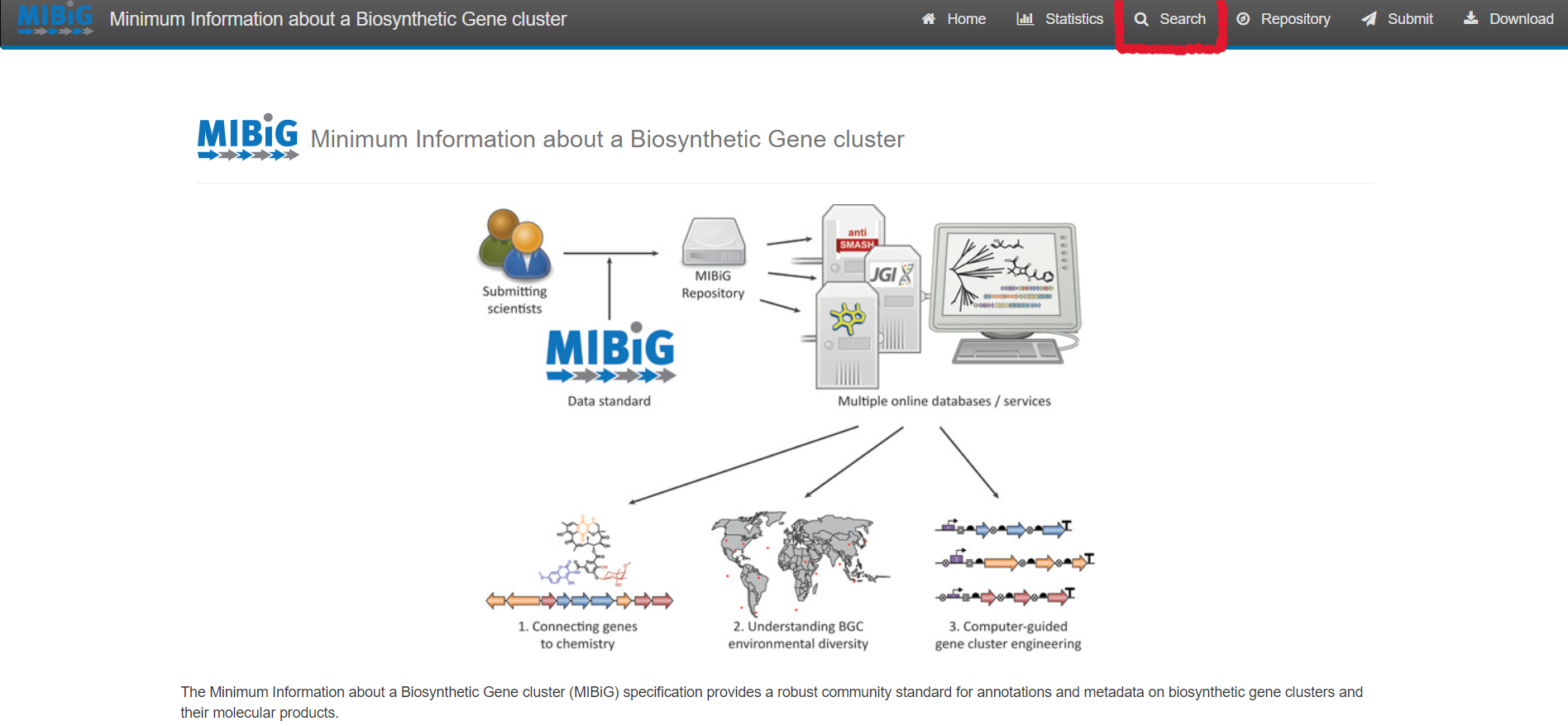
The Minimum Information about a Biosynthetic Gene cluster MIBiG is a database that facilitates consistent and systematic deposition and retrieval of data on biosynthetic gene clusters. MIBiG provides a robust community standard for annotations and metadata on biosynthetic gene clusters and their molecular products. It will empower next-generation research on the biosynthesis, chemistry and ecology of broad classes of societally relevant bioactive secondary metabolites, guided by robust experimental evidence and rich metadata components.

Browsing and Querying in the MIBiG database

Select “Search” on the upper right corner of the menu bar

For simple queries, such as Streptococcus agalactiae or searching for a specific strain you can use the “Simple search” function.

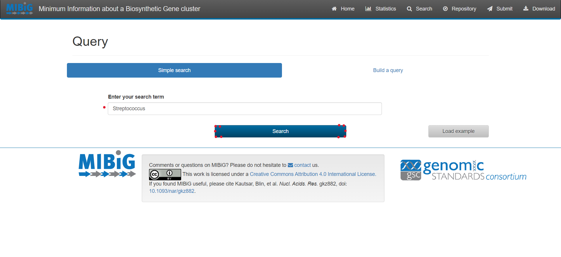
For complex queries, the database also provides a sophisticated query builder that allows querying on all antiSMASH annotations. To enable this function, click on “Build a query”

Results

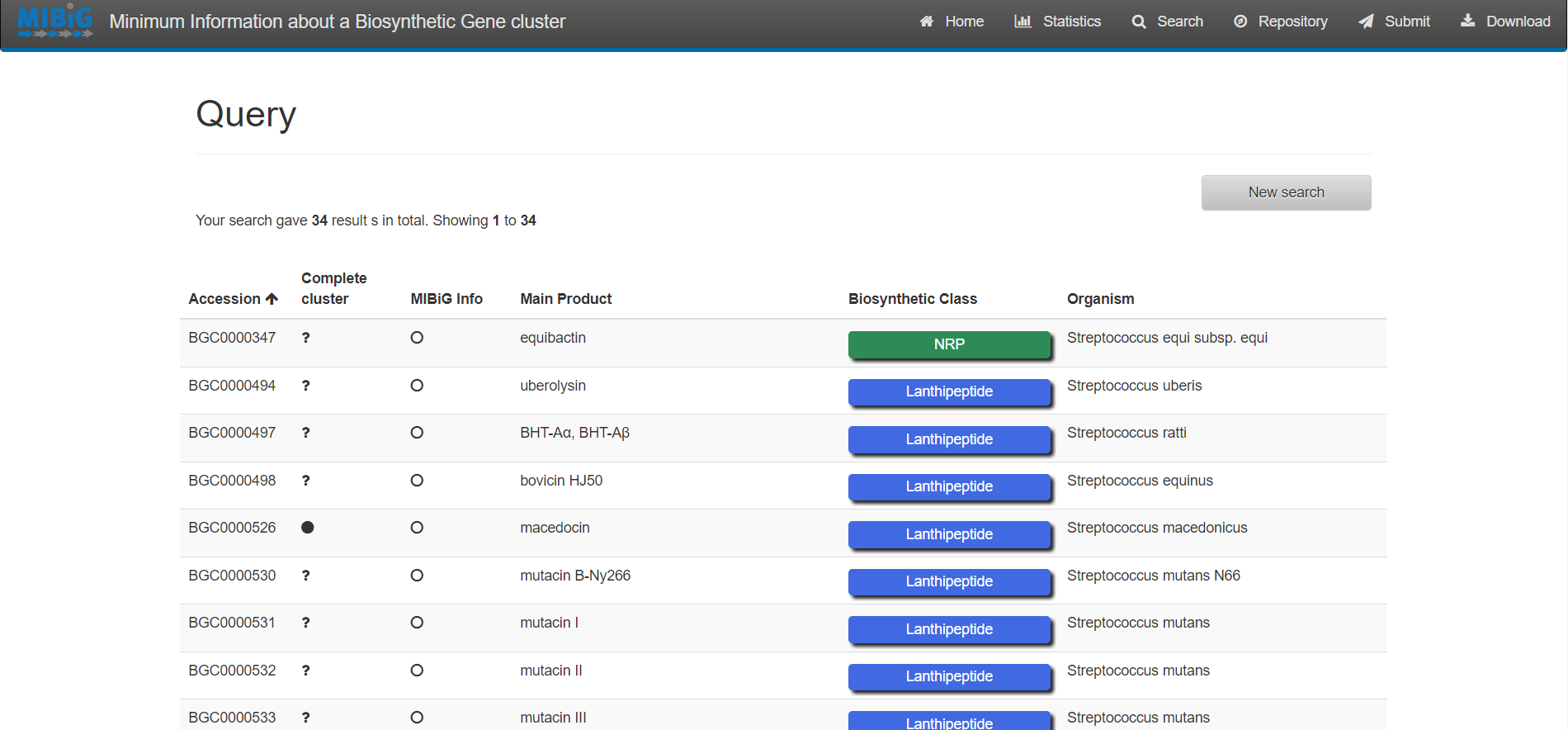
Exercise 1:

Enter to MIBiG and search BGCs from Streptococcus. Search the BGCs that produce the products Thermophilin 1277 and Streptolysin S. Based on the table on MIBiG, which of these organisms has the most complete annotation?

Solution

Streptococcus thermophilus produce Thermophilin 1277 while Streptococcus pyogenes M1 GAS produces Streptolysin S. According to MIBiG metadata Streptolysin S BGC is complete while Thermophilin 1277 is not. So Streptolysin S BGC is better annotated.

antiSMASH database

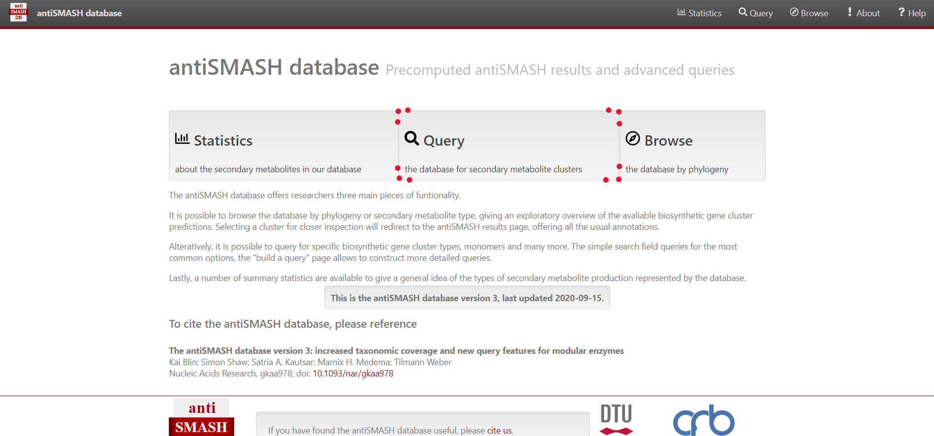
The antiSMASH database provides an easy to use, up-to-date collection of annotated BGC data. It allows to easily perform cross-genome analyses by offering complex queries on the datasets.

Browsing and Querying in the antiSMASH database

Select “Browse” on the top menu bar, alternatively you can select “Query” in the center

For simple queries, such as “Streptococcus” or searching for a specific strain you can use the “Simple search” function.

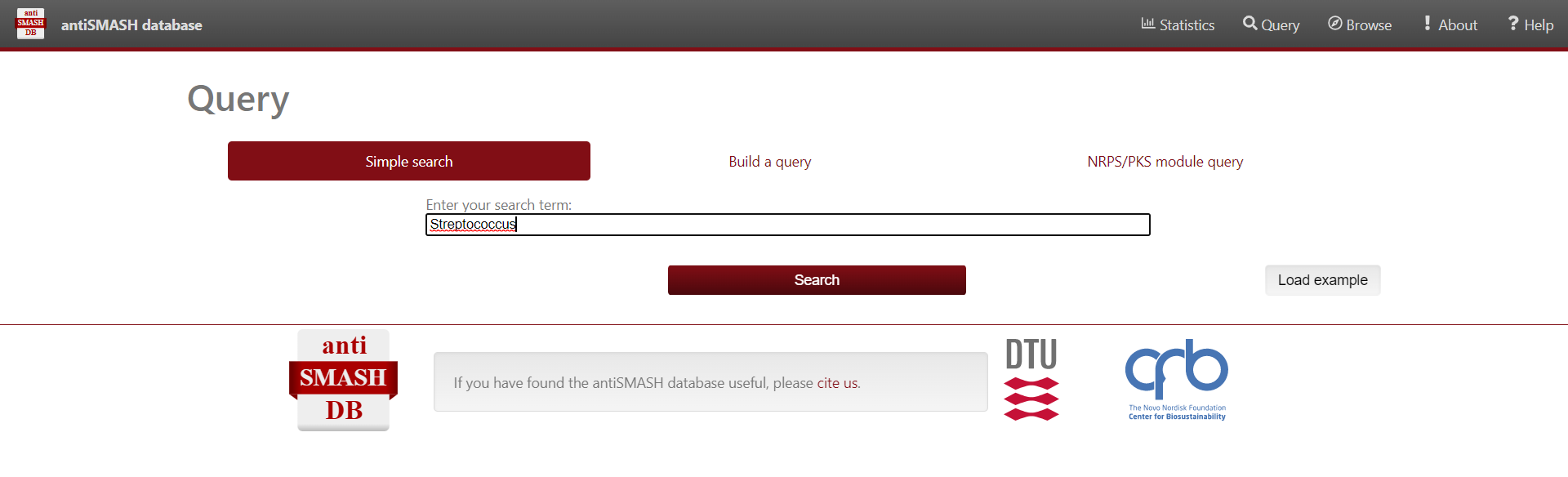
For complex queries, the database also provides a sophisticated query builder that allows querying on all antiSMASH annotations. To enable this function, click on “Build a query”

Results

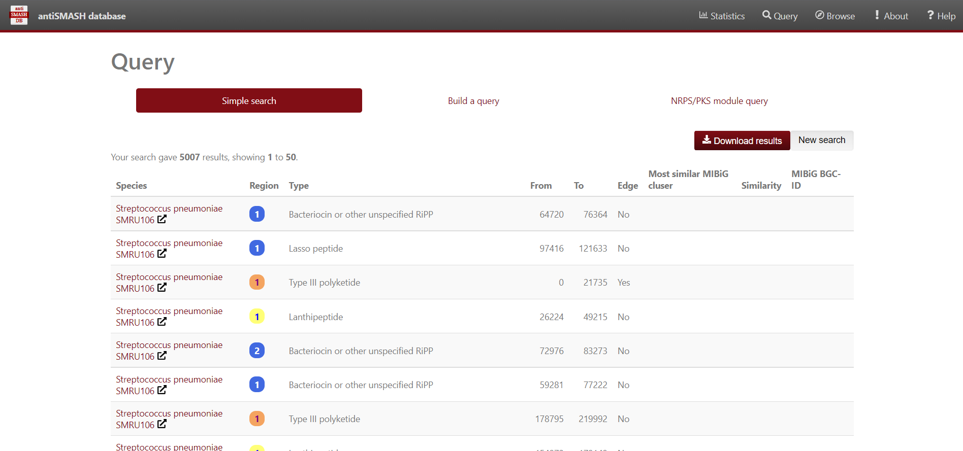
Use antiSMASH database to analyse the BGC contained in the Streptococcus genomes. We’ll use Python to visualize the data. First, import pandas, matplotlib.pyplot and seaborn libraries.

import pandas as pd
import matplotlib.pyplot as plt
import seaborn as sns

Secondly, store in a dataframe variable the content of the Streptococcus predicted BGC downloaded from antiSMASH-db.

data = pd.read_csv("https://raw.githubusercontent.com/AxelRamosGarcia/Genome-Mining/gh-pages/data/antismash_db.csv", sep="\t")
data

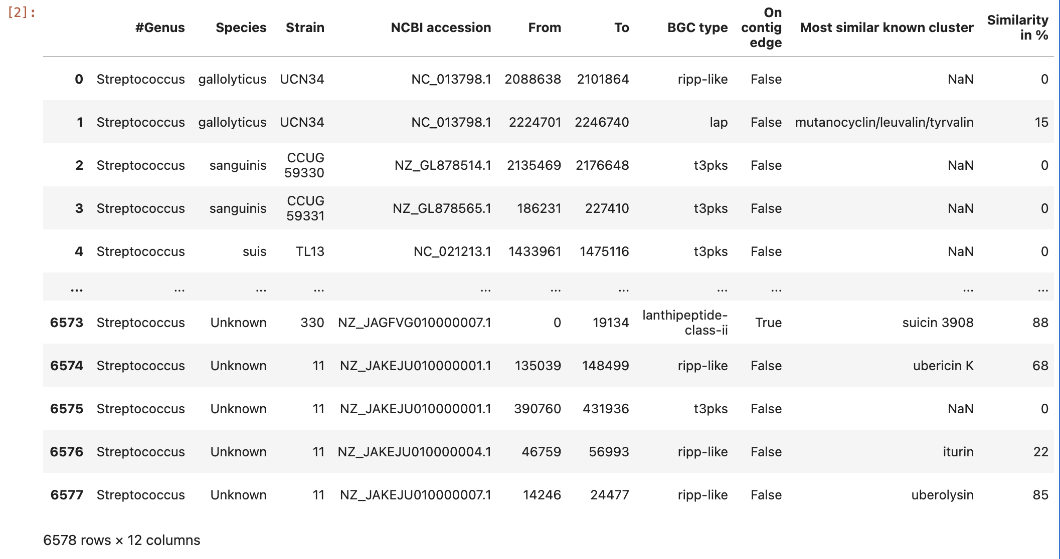
Now, group the data by the variables Species and BGC type:

occurences = data.groupby(["Species", "BGC type"]).size().reset_index(name="Occurrences")

And visualize the content of the ocurrences grouped by species column:

occurences

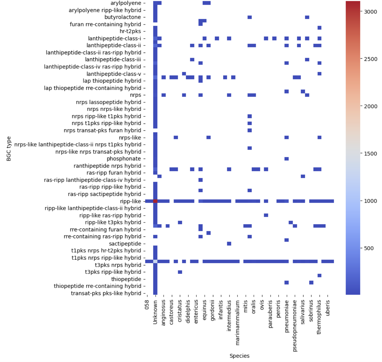
Let’s see our first visualization of the BGC content on a heatmap.

pivot = occurences.pivot(index="BGC type", columns="Species", values="Occurrences")
plt.figure(figsize=(8, 10))
sns.heatmap(pivot, cmap="coolwarm")
plt.show()

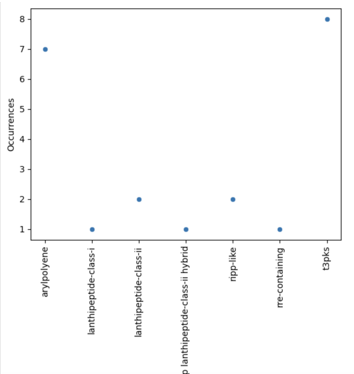
Now, let’s restrict ourselves to S. agalactiae.

agalactiae = occurences[occurences["Species"] == "agalactiae"]
sns.scatterplot(agalactiae, x="BGC type", y="Occurrences")
plt.xticks(rotation="vertical")
plt.show()

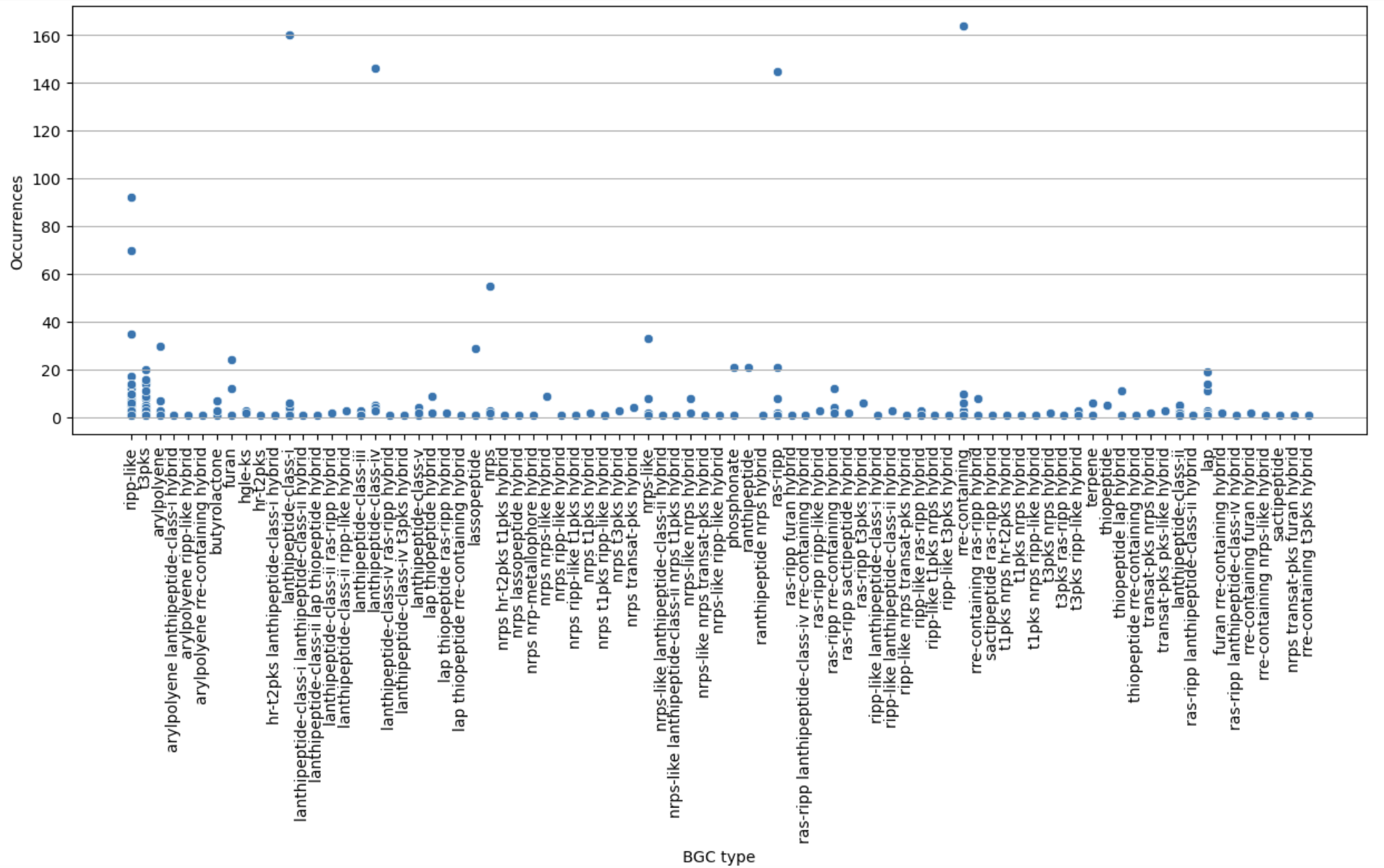
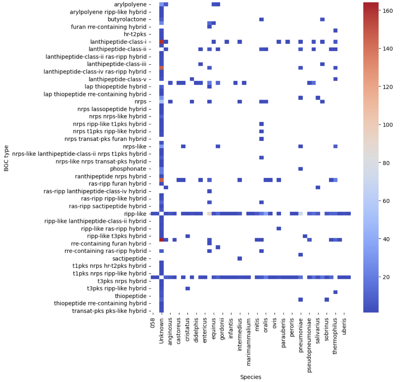
Finally, let’s restrict ourselves to BGC predicted less than 200 times.

filtered = occurences[occurences["Occurrences"] < 200]
plt.figure(figsize=(15, 5))
sns.scatterplot(filtered, x="BGC type", y="Occurrences")
plt.xticks(rotation="vertical")
plt.grid(axis="y")
plt.show()

filtered_pivot = filtered.pivot(index="BGC type", columns="Species", values="Occurrences")
plt.figure(figsize=(8, 10))
sns.heatmap(filtered_pivot, cmap="coolwarm")
plt.show()

Key Points

• MIBiG provides BGCs that have been experimentally tested

• antiSMASH database comprises predicted BGCs of each organism