All in One View
Content from Introduction
Last updated on 2026-05-12 | Edit this page
Overview
Questions
- Why should we care about reproducibility?
- How can
targetshelp us achieve reproducibility?
Objectives
- Explain why reproducibility is important for science
- Describe the features of
targetsthat enhance reproducibility
What is reproducibility?
Reproducibility is the ability for others (including your future self) to reproduce your analysis.
We can only have confidence in the results of scientific analyses if they can be reproduced.
However, reproducibility is not a binary concept (not reproducible vs. reproducible); rather, there is a scale from less reproducible to more reproducible.
targets goes a long ways towards making your analyses
more reproducible.
Other practices you can use to further enhance reproducibility include controlling your computing environment with tools like Docker, conda, or renv, but we don’t have time to cover those in this workshop.
What is targets?
targets is a workflow management package for the R
programming language developed and maintained by Will Landau.
The major features of targets include:
- Automation of workflow
- Caching of workflow steps
- Batch creation of workflow steps
- Parallelization at the level of the workflow
This allows you to do the following:
- return to a project after working on something else and immediately pick up where you left off without confusion or trying to remember what you were doing
- change the workflow, then only re-run the parts that that are affected by the change
- massively scale up the workflow without changing individual functions
… and of course, it will help others reproduce your analysis.
Who should use targets?
targets is by no means the only workflow management
software. There is a large number of similar tools, each with varying
features and use-cases. For example, snakemake is a
popular workflow tool for python, and make is a
tool that has been around for a very long time for automating bash
scripts. targets is designed to work specifically with R,
so it makes the most sense to use it if you primarily use R, or intend
to. If you mostly code with other tools, you may want to consider an
alternative.
The goal of this workshop is to learn how to
use targets to reproducible data analysis in
R.
Where to get more information
targets is a sophisticated package and there is a lot
more to learn that we can cover in this workshop.
Here are some recommended resources for continuing on your
targets journey:
-
The
targetsR package user manual by the author oftargets, Will Landau, should be considered required reading for anyone seriously interested intargets. -
The
targetsdiscussion board is a great place for asking questions and getting help. Before you ask a question though, be sure to read the policy on asking for help. -
The
targetspackage webpage includes documentation of alltargetsfunctions. -
The
tarchetypespackage webpage includes documentation of alltarchetypesfunctions. You will almost certainly usetarchetypesalong withtargets, so it’s good to consult both. -
Reproducible
computation at scale in R with
targetsis a tutorial by Will Landau analyzing customer churn with Keras. -
Recorded
talks and example
projects listed on the
targetsREADME.
About the example dataset
For this workshop, we will analyze an example dataset of measurements taken on adult foraging Adélie, Chinstrap, and Gentoo penguins observed on islands in the Palmer Archipelago, Antarctica.
The data are available from the palmerpenguins R
package. You can get more information about the data by running
?palmerpenguins.

palmerpenguins dataset. Artwork by @allison_horst.The goal of the analysis is to determine the relationship between bill length and depth by using linear models.
We will gradually build up the analysis through this lesson, but you can see the final version at https://github.com/joelnitta/penguins-targets.
- We can only have confidence in the results of scientific analyses if they can be reproduced by others (including your future self)
-
targetshelps achieve reproducibility by automating workflow -
targetsis designed for use with the R programming language - The example dataset for this workshop includes measurements taken on penguins in Antarctica
Content from First targets Workflow
Last updated on 2026-05-12 | Edit this page
Overview
Questions
- What are best practices for organizing analyses?
- What is a
_targets.Rfile for? - What is the content of the
_targets.Rfile? - How do you run a workflow?
Objectives
- Create a project in RStudio
- Explain the purpose of the
_targets.Rfile - Write a basic
_targets.Rfile - Use a
_targets.Rfile to run a workflow
Create a project
About projects
targets uses the “project” concept for organizing
analyses: all of the files needed for a given project are put in a
single folder, the project folder. The project folder has additional
subfolders for organization, such as folders for data, code, and
results.
By using projects, it makes it straightforward to re-orient yourself if you return to an analysis after time spent elsewhere. This wouldn’t be a problem if we only ever work on one thing at a time until completion, but that is almost never the case. It is hard to remember what you were doing when you come back to a project after working on something else (a phenomenon called “context switching”). By using a standardized organization system, you will reduce confusion and lost time… in other words, you are increasing reproducibility!
This workshop will use RStudio, since it also works well with the project organization concept.
Create a project in RStudio
Let’s start a new project using RStudio.
Click “File”, then select “New Project”.
This will open the New Project Wizard, a set of menus to help you set up the project.
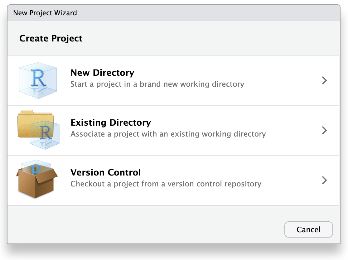
In the Wizard, click the first option, “New Directory”, since we are making a brand-new project from scratch. Click “New Project” in the next menu. In “Directory name”, enter a name that helps you remember the purpose of the project, such as “targets-demo” (follow best practices for naming files and folders). Under “Create project as a subdirectory of…”, click the “Browse” button to select a directory to put the project. We recommend putting it on your Desktop so you can easily find it.
You can leave “Create a git repository” and “Use renv with this project” unchecked, but these are both excellent tools to improve reproducibility, and you should consider learning them and using them in the future, if you don’t already. They can be enabled at any later time, so you don’t need to worry about trying to use them immediately.
Once you work through these steps, your RStudio session should look like this:
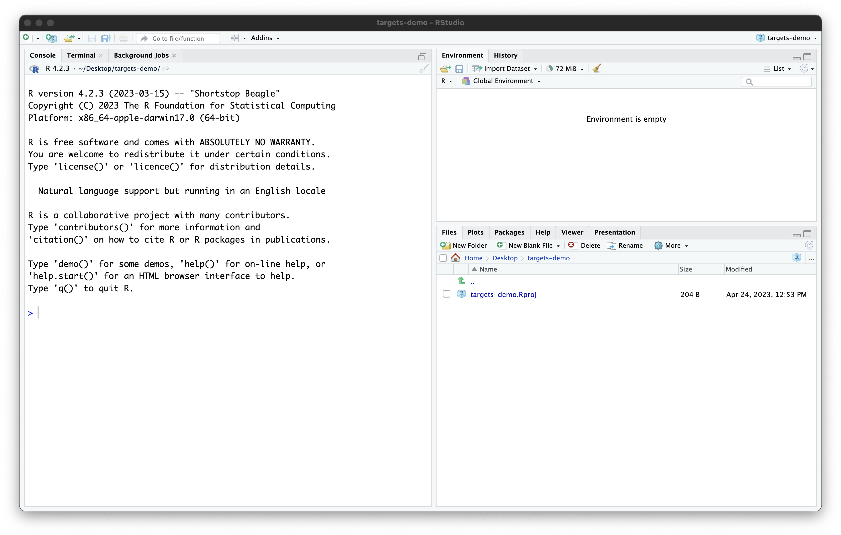
Our project now contains a single file, created by RStudio:
targets-demo.Rproj. You should not edit this file by hand.
Its purpose is to tell RStudio that this is a project folder and to
store some RStudio settings (if you use version-control software, it is
OK to commit this file). Also, you can open the project by double
clicking on the .Rproj file in your file explorer (try it
by quitting RStudio then navigating in your file browser to your
Desktop, opening the “targets-demo” folder, and double clicking
targets-demo.Rproj).
OK, now that our project is set up, we are (almost) ready to start
using targets!
Background: non-targets version
First though, to get familiar with the functions and packages we’ll
use, let’s run the code like you would in a “normal” R script without
using targets.
Recall that we are using the palmerpenguins R package to
obtain the data. This package actually includes two variations of the
dataset: one is an external CSV file with the raw data, and another is
the cleaned data loaded into R. In real life you are probably have
externally stored raw data, so let’s use the raw penguin
data as the starting point for our analysis too.
The path_to_file() function in
palmerpenguins provides the path to the raw data CSV file
(it is inside the palmerpenguins R package source code that
you downloaded to your computer when you installed the package).
R
library(palmerpenguins)
OUTPUT
Attaching package: 'palmerpenguins'OUTPUT
The following objects are masked from 'package:datasets':

    penguins, penguins_raw
R
# Get path to CSV file
penguins_csv_file <- path_to_file("penguins_raw.csv")

penguins_csv_file
OUTPUT
[1] "/home/runner/.local/share/renv/cache/v5/linux-ubuntu-jammy/R-4.5/x86_64-pc-linux-gnu/palmerpenguins/0.1.1/6c6861efbc13c1d543749e9c7be4a592/palmerpenguins/extdata/penguins_raw.csv"We will use the tidyverse set of packages for loading
and manipulating the data. We don’t have time to cover all the details
about using tidyverse now, but if you want to learn more
about it, please see the “Manipulating,
analyzing and exporting data with tidyverse” lesson, or the
Carpentry incubator lesson R
and the tidyverse for working with datasets.
Let’s load the data with read_csv().
R
library(tidyverse)

# Read CSV file into R
penguins_data_raw <- read_csv(penguins_csv_file)

penguins_data_raw
OUTPUT
Rows: 344 Columns: 17
── Column specification ────────────────────────────────────────────────────────
Delimiter: ","
chr  (9): studyName, Species, Region, Island, Stage, Individual ID, Clutch C...
dbl  (7): Sample Number, Culmen Length (mm), Culmen Depth (mm), Flipper Leng...
date (1): Date Egg

ℹ Use `spec()` to retrieve the full column specification for this data.
ℹ Specify the column types or set `show_col_types = FALSE` to quiet this message.
OUTPUT
# A tibble: 344 × 17
   studyName `Sample Number` Species         Region Island Stage `Individual ID`
   <chr>               <dbl> <chr>           <chr>  <chr>  <chr> <chr>
 1 PAL0708                 1 Adelie Penguin… Anvers Torge… Adul… N1A1
 2 PAL0708                 2 Adelie Penguin… Anvers Torge… Adul… N1A2
 3 PAL0708                 3 Adelie Penguin… Anvers Torge… Adul… N2A1
 4 PAL0708                 4 Adelie Penguin… Anvers Torge… Adul… N2A2
 5 PAL0708                 5 Adelie Penguin… Anvers Torge… Adul… N3A1
 6 PAL0708                 6 Adelie Penguin… Anvers Torge… Adul… N3A2
 7 PAL0708                 7 Adelie Penguin… Anvers Torge… Adul… N4A1
 8 PAL0708                 8 Adelie Penguin… Anvers Torge… Adul… N4A2
 9 PAL0708                 9 Adelie Penguin… Anvers Torge… Adul… N5A1
10 PAL0708                10 Adelie Penguin… Anvers Torge… Adul… N5A2
# ℹ 334 more rows
# ℹ 10 more variables: `Clutch Completion` <chr>, `Date Egg` <date>,
#   `Culmen Length (mm)` <dbl>, `Culmen Depth (mm)` <dbl>,
#   `Flipper Length (mm)` <dbl>, `Body Mass (g)` <dbl>, Sex <chr>,
#   `Delta 15 N (o/oo)` <dbl>, `Delta 13 C (o/oo)` <dbl>, Comments <chr>
We see the raw data has some awkward column names with spaces (these are hard to type out and can easily lead to mistakes in the code), and far more columns than we need. For the purposes of this analysis, we only need species name, bill length, and bill depth. In the raw data, the rather technical term “culmen” is used to refer to the bill.

Let’s clean up the data to make it easier to use for downstream analyses. We will also remove any rows with missing data, because this could cause errors for some functions later.
R
# Clean up raw data
penguins_data <- penguins_data_raw |>
  # Rename columns for easier typing and
  # subset to only the columns needed for analysis
  select(
    species = Species,
    bill_length_mm = `Culmen Length (mm)`,
    bill_depth_mm = `Culmen Depth (mm)`
  ) |>
  # Delete rows with missing data
  drop_na()

penguins_data
OUTPUT
# A tibble: 342 × 3
   species                             bill_length_mm bill_depth_mm
   <chr>                                        <dbl>         <dbl>
 1 Adelie Penguin (Pygoscelis adeliae)           39.1          18.7
 2 Adelie Penguin (Pygoscelis adeliae)           39.5          17.4
 3 Adelie Penguin (Pygoscelis adeliae)           40.3          18
 4 Adelie Penguin (Pygoscelis adeliae)           36.7          19.3
 5 Adelie Penguin (Pygoscelis adeliae)           39.3          20.6
 6 Adelie Penguin (Pygoscelis adeliae)           38.9          17.8
 7 Adelie Penguin (Pygoscelis adeliae)           39.2          19.6
 8 Adelie Penguin (Pygoscelis adeliae)           34.1          18.1
 9 Adelie Penguin (Pygoscelis adeliae)           42            20.2
10 Adelie Penguin (Pygoscelis adeliae)           37.8          17.1
# ℹ 332 more rows
We have not run the full analysis yet, but this is enough to get us
started with the transition to using targets.
targets version
About the _targets.R file
One major difference between a typical R data analysis and a
targets project is that the latter must include a special
file, called _targets.R in the main project folder (the
“project root”).
The _targets.R file includes the specification of the
workflow: these are the directions for R to run your analysis, kind of
like a recipe. By using the _targets.R file, you
won’t have to remember to run specific scripts in a certain
order; instead, R will do it for you! This is a huge
win, both for your future self and anybody else trying to
reproduce your analysis.
Writing the initial _targets.R file
We will now start to write a _targets.R file.
Fortunately, targets comes with a function to help us do
this.
In the R console, first load the targets package with
library(targets), then run the command
tar_script().
R
library(targets)
tar_script()
Nothing will happen in the console, but in the file viewer, you
should see a new file, _targets.R appear. Open it using the
File menu or by clicking on it.
R
library(targets)
# This is an example _targets.R file. Every
# {targets} pipeline needs one.
# Use tar_script() to create _targets.R and tar_edit()
# to open it again for editing.
# Then, run tar_make() to run the pipeline
# and tar_read(data_summary) to view the results.

# Define custom functions and other global objects.
# This is where you write source(\"R/functions.R\")
# if you keep your functions in external scripts.
summarize_data <- function(dataset) {
  colMeans(dataset)
}

# Set target-specific options such as packages:
# tar_option_set(packages = "utils") # nolint

# End this file with a list of target objects.
list(
  tar_target(data, data.frame(x = sample.int(100), y = sample.int(100))),
  tar_target(data_summary, summarize_data(data)) # Call your custom functions.
)
Don’t worry about the details of this file. Instead, notice that that it includes three main parts:
- Loading packages with
library() - Defining a custom function with
function() - Defining a list with
list().
You may not have used function() before. If not, that’s
OK; we will cover this in more detail in the next episode, so we will ignore it for
now.
The last part, the list, is the most important part
of the _targets.R file. It defines the steps in the
workflow. The _targets.R file must always end with
this list.
Furthermore, each item in the list is a call of the
tar_target() function. The first argument of
tar_target() is name of the target to build, and the second
argument is the command used to build it. Note that the name of the
target is unquoted, that is, it is written without any
surrounding quotation marks.
Modifying _targets.R to run the example analysis
First, let’s load all of the packages we need for our workflow. Add
library(tidyverse) and library(palmerpenguins)
to the top of _targets.R after
library(targets).
Next, we can delete the function() statement since we
won’t be using that just yet (we will come back to custom functions
soon!).
The last, and trickiest, part is correctly defining the workflow in the list at the end of the file.
From the
non-targets version, you can see we have three steps so
far:
- Define the path to the CSV file with the raw penguins data.
- Read the CSV file.
- Clean the raw data.
Each of these will be one item in the list. Furthermore, we need to
write each item using the tar_target() function. Recall
that we write the tar_target() function by writing the
name of the target to build first and the
command to build it second.
Choosing good target names
The name of each target could be anything you like, but it is strongly recommended to choose names that reflect what the target actually contains.
For example, penguins_data_raw for the raw data loaded
from the CSV file and not x.
Your future self will thank you!
Challenge: Use tar_target()
Can you use tar_target() to define the first step in the
workflow (setting the path to the CSV file with the penguins data)?
R
tar_target(name = penguins_csv_file, command = path_to_file("penguins_raw.csv"))
The first two arguments of tar_target() are the
name of the target, followed by the
command to build it.
These arguments are used so frequently we will typically omit the argument names, instead writing it like this:
R
tar_target(penguins_csv_file, path_to_file("penguins_raw.csv"))
Now that we’ve seen how to define the first target, let’s continue and add the rest.
Once you’ve done that, this is how _targets.R should
look:
R
library(targets)
library(tidyverse)
library(palmerpenguins)

list(
  tar_target(penguins_csv_file, path_to_file("penguins_raw.csv")),
  tar_target(
    penguins_data_raw,
    read_csv(penguins_csv_file, show_col_types = FALSE)
  ),
  tar_target(
    penguins_data,
    penguins_data_raw |>
      select(
        species = Species,
        bill_length_mm = `Culmen Length (mm)`,
        bill_depth_mm = `Culmen Depth (mm)`
      ) |>
      drop_na()
  )
)
I have set show_col_types = FALSE in
read_csv() because we know from the earlier code that the
column types were set correctly by default (character for species and
numeric for bill length and depth), so we don’t need to see the warning
it would otherwise issue.
Run the workflow
Now that we have a workflow, we can run it with the
tar_make() function. Try running it, and you should see
something like this:
R
tar_make()
OUTPUT
Attaching package: ‘palmerpenguins’

The following objects are masked from ‘package:datasets’:

    penguins, penguins_raw

+ penguins_csv_file dispatched
✔ penguins_csv_file completed [1ms, 190 B]
+ penguins_data_raw dispatched
✔ penguins_data_raw completed [102ms, 10.40 kB]
+ penguins_data dispatched
✔ penguins_data completed [14ms, 1.61 kB]
✔ ended pipeline [342ms, 3 completed, 0 skipped]
Congratulations, you’ve run your first workflow with
targets!
The workflow cannot be run interactively
You may be used to running R code interactively by selecting lines and pressing the “Run” button (or using the keyboard shortcut) in RStudio or your IDE of choice.
You could run the list at the of _targets.R
this way, but it will not execute the workflow (it will return a list
instead).
The only way to run the workflow is with
tar_make().
You do not need to select and run anything interactively in
_targets.R. In fact, you do not even need to have the
_targets.R file open to run the workflow with
tar_make()—try it for yourself!
Similarly, you must not write tar_make() in the
_targets.R file; you should only use
tar_make() as a direct command at the R console.
Remember, now that we are using targets, the
only thing you need to do to replicate your analysis is run
tar_make().
This is true no matter how long or complicated your analysis becomes.
- Projects help keep our analyses organized so we can easily re-run them later
- Use the RStudio Project Wizard to create projects
- The
_targets.Rfile is a special file that must be included in alltargetsprojects, and defines the worklow - Use
tar_script()to create a default_targets.Rfile - Use
tar_make()to run the workflow
Content from A Brief Introduction to Functions
Last updated on 2026-05-12 | Edit this page
Overview
Questions
- What are functions?
- Why should we know how to write them?
- What are the main components of a function?
Objectives
- Understand the usefulness of custom functions
- Understand the basic concepts around writing functions
About functions
Functions in R are something we are used to thinking of as something that comes from a package. You find, install and use specialized functions from packages to get your work done.
But you can, and arguably should, be writing your own functions too! Functions are a great way of making it easy to repeat the same operation but with different settings. How many times have you copy-pasted the exact same code in your script, only to change a couple of things (a variable, an input etc.) before running it again? Only to then discover that there was an error in the code, and when you fix it, you need to remember to do so in all the places where you copied that code.
Through writing functions you can reduce this back and forth, and create a more efficient workflow for yourself. When you find the bug, you fix it in a single place, the function you made, and each subsequent call of that function will now be fixed.
Furthermore, targets makes extensive use of custom
functions, so a basic understanding of how they work is very important
to successfully using it.
Writing a function
There is not much difference between writing your own function and writing other code in R, you are still coding with R! Let’s imagine we want to convert the millimeter measurements in the penguins data to centimeters.
R
library(palmerpenguins)
library(tidyverse)

penguins |>
  mutate(
    bill_length_cm = bill_length_mm / 10,
    bill_depth_cm = bill_depth_mm / 10
  )
OUTPUT
# A tibble: 344 × 10
   species island    bill_length_mm bill_depth_mm flipper_length_mm body_mass_g
   <fct>   <fct>              <dbl>         <dbl>             <int>       <int>
 1 Adelie  Torgersen           39.1          18.7               181        3750
 2 Adelie  Torgersen           39.5          17.4               186        3800
 3 Adelie  Torgersen           40.3          18                 195        3250
 4 Adelie  Torgersen           NA            NA                  NA          NA
 5 Adelie  Torgersen           36.7          19.3               193        3450
 6 Adelie  Torgersen           39.3          20.6               190        3650
 7 Adelie  Torgersen           38.9          17.8               181        3625
 8 Adelie  Torgersen           39.2          19.6               195        4675
 9 Adelie  Torgersen           34.1          18.1               193        3475
10 Adelie  Torgersen           42            20.2               190        4250
# ℹ 334 more rows
# ℹ 4 more variables: sex <fct>, year <int>, bill_length_cm <dbl>,
#   bill_depth_cm <dbl>
This is not a complicated operation, but we might want to make a convenient custom function that can do this conversion for us anyways.
To write a function, you need to use the function()
function. With this function we provide what will be the input arguments
of the function inside its parentheses, and what the function will
subsequently do with those input arguments in curly braces
{} after the function parentheses. The object name we
assign this to, will become the function’s name.
R
my_function <- function(argument1, argument2) {
  # the things the function will do
}
# call the function
my_function(1, "something")
For our mm to cm conversion the function would look like so:
R
mm2cm <- function(x) {
  x / 10
}
Our custom function will now transform any numerical input by dividing it by 10.
Let’s try it out:
R
penguins |>
  mutate(
    bill_length_cm = mm2cm(bill_length_mm),
    bill_depth_cm = mm2cm(bill_depth_mm)
  )
OUTPUT
# A tibble: 344 × 10
   species island    bill_length_mm bill_depth_mm flipper_length_mm body_mass_g
   <fct>   <fct>              <dbl>         <dbl>             <int>       <int>
 1 Adelie  Torgersen           39.1          18.7               181        3750
 2 Adelie  Torgersen           39.5          17.4               186        3800
 3 Adelie  Torgersen           40.3          18                 195        3250
 4 Adelie  Torgersen           NA            NA                  NA          NA
 5 Adelie  Torgersen           36.7          19.3               193        3450
 6 Adelie  Torgersen           39.3          20.6               190        3650
 7 Adelie  Torgersen           38.9          17.8               181        3625
 8 Adelie  Torgersen           39.2          19.6               195        4675
 9 Adelie  Torgersen           34.1          18.1               193        3475
10 Adelie  Torgersen           42            20.2               190        4250
# ℹ 334 more rows
# ℹ 4 more variables: sex <fct>, year <int>, bill_length_cm <dbl>,
#   bill_depth_cm <dbl>
Congratulations, you’ve created and used your first custom function!
Make a function from existing code
Many times, we might already have a piece of code that we’d like to
use to create a function. For instance, we’ve copy-pasted a section of
code several times and realize that this piece of code is repetitive, so
a function is in order. Or, you are converting your workflow to
targets, and need to change your script into a series of
functions that targets will call.
Recall the code snippet we had to clean our penguins data:
R
penguins_data_raw |>
  select(
    species = Species,
    bill_length_mm = `Culmen Length (mm)`,
    bill_depth_mm = `Culmen Depth (mm)`
  ) |>
  drop_na()
We need to adapt this code to become a function, and this function needs a single argument, which is the dataset it should clean.
It should look like this:
R
clean_penguin_data <- function(penguins_data_raw) {
  penguins_data_raw |>
    select(
      species = Species,
      bill_length_mm = `Culmen Length (mm)`,
      bill_depth_mm = `Culmen Depth (mm)`
    ) |>
    drop_na()
}
Add this function to _targets.R after the part where you
load packages with library() and before the list at the
end.
RStudio function extraction
RStudio also has a handy helper to extract a function from a piece of code. Once you have basic familiarity with functions, it may help you figure out the necessary input when turning code into a function.
To use it, highlight the piece of code you want to make into a
function. In our case that is the entire pipeline from
penguins_data_raw to the drop_na() statement.
Once you have done this, in RStudio go to the “Code” section in the top
bar, and select “Extract function” from the list. A prompt will open
asking you to hit enter, and you should have the following code in your
script where the cursor was.
This function will not work however, because it contains more stuff
than is needed as an argument. This is because tidyverse uses
non-standard evaluation, and we can write unquoted column names inside
the select(). The function extractor thinks that all
unquoted (or back-ticked) text in the code is a reference to an object.
You will need to do some manual cleaning to get the function working,
which is why its more convenient if you have a little experience with
functions already.
Challenge: Write a function that takes a numerical vector and returns its mean divided by 10.
R
vecmean <- function(x) {
  mean(x) / 10
}
Using functions in the workflow
Now that we’ve defined our custom data cleaning function, we can put it to use in the workflow.
Can you see how this might be done?
We need to delete the corresponding code from the last
tar_target() and replace it with a call to the new
function.
Modify the workflow to look like this:
R
library(targets)
library(tidyverse)
library(palmerpenguins)

clean_penguin_data <- function(penguins_data_raw) {
  penguins_data_raw |>
    select(
      species = Species,
      bill_length_mm = `Culmen Length (mm)`,
      bill_depth_mm = `Culmen Depth (mm)`
    ) |>
    drop_na()
}

list(
  tar_target(penguins_csv_file, path_to_file("penguins_raw.csv")),
  tar_target(penguins_data_raw, read_csv(
    penguins_csv_file, show_col_types = FALSE)),
  tar_target(penguins_data, clean_penguin_data(penguins_data_raw))
)
We should run the workflow again with tar_make() to make
sure it is up-to-date:
OUTPUT
Attaching package: ‘palmerpenguins’

The following objects are masked from ‘package:datasets’:

    penguins, penguins_raw
R
tar_make()
OUTPUT
Attaching package: ‘palmerpenguins’

The following objects are masked from ‘package:datasets’:

    penguins, penguins_raw

+ penguins_data dispatched
✔ penguins_data completed [25ms, 1.61 kB]
✔ ended pipeline [192ms, 1 completed, 2 skipped]
We will learn more soon about the messages that
targets() prints out.
Functions make it easier to reason about code
Notice that now the list of targets at the end is starting to look like a high-level summary of your analysis.
This is another advantage of using custom functions: functions allows us to separate the details of each workflow step from the overall workflow.
To understand the overall workflow, you don’t need to know all of the details about how the data were cleaned; you just need to know that there was a cleaning step. On the other hand, if you do need to go back and delve into the specifics of the data cleaning, you only need to pay attention to what happens inside that function, and you can ignore the rest of the workflow. This makes it easier to reason about the code, and will lead to fewer bugs and ultimately save you time and mental energy.
Here we have only scratched the surface of functions, and you will likely need to get more help in learning about them. For more information, we recommend reading this episode in the R Novice lesson from Carpentries that is all about functions.
- Functions are crucial when repeating the same code many times with minor differences
- RStudio’s “Extract function” tool can help you get started with converting code into functions
- Functions are an essential part of how
targetsworks.
Content from Loading Workflow Objects
Last updated on 2026-05-12 | Edit this page
Overview
Questions
- Where does the workflow happen?
- How can we inspect the objects built by the workflow?
Objectives
- Explain where
targetsruns the workflow and why - Be able to load objects built by the workflow into your R session
Where does the workflow happen?
So we just finished running our workflow. Now you probably want to
look at its output. But, if we just call the name of the object (for
example, penguins_data), we get an error.
R
penguins_data
ERROR
Error: object 'penguins_data' not foundWhere are the results of our workflow?
We don’t see the workflow results because targets
runs the workflow in a separate R session that we can’t
interact with. This is for reproducibility—the objects built by the
workflow should only depend on the code in your project, not any
commands you may have interactively given to R.
Fortunately, targets has two functions that can be used
to load objects built by the workflow into our current session,
tar_load() and tar_read(). Let’s see how these
work.
tar_load()
tar_load() loads an object built by the workflow into
the current session. Its first argument is the name of the object you
want to load. Let’s use this to load penguins_data and get
an overview of the data with summary().
OUTPUT
Attaching package: ‘palmerpenguins’

The following objects are masked from ‘package:datasets’:

    penguins, penguins_raw
R
tar_load(penguins_data)
summary(penguins_data)
OUTPUT
   species          bill_length_mm  bill_depth_mm
 Length:342         Min.   :32.10   Min.   :13.10
 Class :character   1st Qu.:39.23   1st Qu.:15.60
 Mode  :character   Median :44.45   Median :17.30
                    Mean   :43.92   Mean   :17.15
                    3rd Qu.:48.50   3rd Qu.:18.70
                    Max.   :59.60   Max.   :21.50
Note that tar_load() is used for its
side-effect—loading the desired object into the current
R session. It doesn’t actually return a value.
tar_read()
tar_read() is similar to tar_load() in that
it is used to retrieve objects built by the workflow, but unlike
tar_load(), it returns them directly as output.
Let’s try it with penguins_csv_file.
R
tar_read(penguins_csv_file)
OUTPUT
[1] "/home/runner/.local/share/renv/cache/v5/linux-ubuntu-jammy/R-4.5/x86_64-pc-linux-gnu/palmerpenguins/0.1.1/6c6861efbc13c1d543749e9c7be4a592/palmerpenguins/extdata/penguins_raw.csv"We immediately see the contents of penguins_csv_file.
But it has not been loaded into the environment. If you try to run
penguins_csv_file now, you will get an error:
R
penguins_csv_file
ERROR
Error: object 'penguins_csv_file' not foundWhen to use which function
tar_load() tends to be more useful when you want to load
objects and do things with them. tar_read() is more useful
when you just want to immediately inspect an object.
The targets cache
If you close your R session, then re-start it and use
tar_load() or tar_read(), you will notice that
it can still load the workflow objects. In other words, the workflow
output is saved across R sessions. How is this
possible?
You may have noticed a new folder has appeared in your project,
called _targets. This is the targets
cache. It contains all of the workflow output; that is how we
can load the targets built by the workflow even after quitting then
restarting R.
You should not edit the contents of the cache by hand (with one exception). Doing so would make your analysis non-reproducible.
The one exception to this rule is a special subfolder called
_targets/user. This folder does not exist by default. You
can create it if you want, and put whatever you want inside.
Generally, _targets/user is a good place to store files
that are not code, like data and output.
Note that if you don’t have anything in _targets/user
that you need to keep around, it is possible to “reset” your workflow by
simply deleting the entire _targets folder. Of course, this
means you will need to run everything over again, so don’t do this
lightly!
-
targetsworkflows are run in a separate, non-interactive R session -
tar_load()loads a workflow object into the current R session -
tar_read()reads a workflow object and returns its value - The
_targetsfolder is the cache and generally should not be edited by hand
Content from The Workflow Lifecycle
Last updated on 2026-05-12 | Edit this page
Overview
Questions
- What happens if we re-run a workflow?
- How does
targetsknow what steps to re-run? - How can we inspect the state of the workflow?
Objectives
- Explain how
targetshelps increase efficiency - Be able to inspect a workflow to see what parts are outdated
Re-running the workflow
One of the features of targets is that it maximizes
efficiency by only running the parts of the workflow that need to be
run.
This is easiest to understand by trying it yourself. Let’s try running the workflow again:
OUTPUT
Attaching package: ‘palmerpenguins’

The following objects are masked from ‘package:datasets’:

    penguins, penguins_raw
R
tar_make()
OUTPUT
Attaching package: ‘palmerpenguins’

The following objects are masked from ‘package:datasets’:

    penguins, penguins_raw

✔ skipped pipeline [132ms, 3 skipped]
Remember how the first time we ran the pipeline, targets
printed out a list of each target as it was being built?
This time, it tells us it is skipping those targets; they have already been built, so there’s no need to run that code again.
Remember, the fastest code is the code you don’t have to run!
Re-running the workflow after modification
What happens when we change one part of the workflow then run it again?
Say that we decide the species names should be shorter. Right now they include the common name and the scientific name, but we really only need the first part of the common name to distinguish them.
Edit _targets.R so that the
clean_penguin_data() function looks like this:
R
clean_penguin_data <- function(penguins_data_raw) {
  penguins_data_raw |>
    select(
      species = Species,
      bill_length_mm = `Culmen Length (mm)`,
      bill_depth_mm = `Culmen Depth (mm)`
    ) |>
    drop_na() |>
    # Split "species" apart on spaces, and only keep the first word
    separate(species, into = "species", extra = "drop")
}
Then run it again.
OUTPUT
Attaching package: ‘palmerpenguins’

The following objects are masked from ‘package:datasets’:

    penguins, penguins_raw
R
tar_make()
OUTPUT
Attaching package: ‘palmerpenguins’

The following objects are masked from ‘package:datasets’:

    penguins, penguins_raw

+ penguins_data dispatched
✔ penguins_data completed [23ms, 1.49 kB]
✔ ended pipeline [242ms, 1 completed, 2 skipped]
What happened?
This time, it skipped penguins_csv_file and
penguins_data_raw and only ran
penguins_data.
Of course, since our example workflow is so short we don’t even notice the amount of time saved. But imagine using this in a series of computationally intensive analysis steps. The ability to automatically skip steps results in a massive increase in efficiency.
Challenge 1: Inspect the output
How can you inspect the contents of penguins_data?
With tar_read(penguins_data) or by running
tar_load(penguins_data) followed by
penguins_data.
Under the hood
How does targets keep track of which targets are
up-to-date vs. outdated?
For each target in the workflow (items in the list at the end of the
_targets.R file) and any custom functions used in the
workflow, targets calculates a hash value,
or unique combination of letters and digits that represents an object in
the computer’s memory. You can think of the hash value (or “hash” for
short) as a unique fingerprint for a target or
function.
The first time your run tar_make(), targets
calculates the hashes for each target and function as it runs the code
and stores them in the targets cache (the _targets folder).
Then, for each subsequent call of tar_make(), it calculates
the hashes again and compares them to the stored values. It detects
which have changed, and this is how it knows which targets are out of
date.
Where the hashes live
If you are curious about what the hashes look like, you can see them
in the file _targets/meta/meta, but do not edit
this file by hand—that would ruin your workflow!
This information is used in combination with the dependency relationships (in other words, how each target depends on the others) to re-run the workflow in the most efficient way possible: code is only run for targets that need to be re-built, and others are skipped.
Visualizing the workflow
Typically, you will be making edits to various places in your code, adding new targets, and running the workflow periodically. It is good to be able to visualize the state of the workflow.
This can be done with tar_visnetwork()
R
tar_visnetwork()
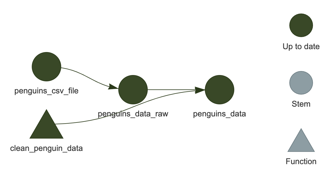
You should see the network show up in the plot area of RStudio.
It is an HTML widget, so you can zoom in and out (this isn’t important for the current example since it is so small, but is useful for larger, “real-life” workflows).
Here, we see that all of the targets are dark green, indicating that they are up-to-date and would be skipped if we were to run the workflow again.
Installing visNetwork
You may encounter an error message
The package "visNetwork" is required.
In this case, install it first with
install.packages("visNetwork").
Challenge 2: What else can the visualization tell us?
Modify the workflow in _targets.R, then run
tar_visnetwork() again without running
tar_make(). What color indicates that a target is out of
date?
Light blue indicates the target is out of date.
Depending on how you modified the code, any or all of the targets may now be light blue.
‘Outdated’ does not always mean ‘will be run’
Just because a target appears as light blue (is “outdated”) in the network visualization, this does not guarantee that it will be re-built during the next run. Rather, it means that at least of one the targets that it depends on has changed.
For example, if the workflow state looked like this:
A -> B* -> C -> D
where the * indicates that B has changed
compared to the last time the workflow was run, the network
visualization will show B, C, and
D all as light blue.
But if re-running the workflow results in the exact same value for
C as before, D will not be re-run (will be
“skipped”).
Most of the time, a single change will cascade to the rest of the
downstream targets and cause them to be re-built, but this is not always
the case. targets has no way of knowing ahead of time what
the actual output will be, so it cannot provide a network visualization
that completely predicts the future!
Other ways to check workflow status
The visualization is very useful, but sometimes you may be working on a server that doesn’t provide graphical output, or you just want a quick textual summary of the workflow. There are some other useful functions that can do that.
tar_outdated() lists only the outdated targets; that is,
targets that will be built during the next run, or depend on such a
target. If everything is up to date, it will return a zero-length
character vector (character(0)).
R
tar_outdated()
OUTPUT
Attaching package: ‘palmerpenguins’

The following objects are masked from ‘package:datasets’:

    penguins, penguins_raw
OUTPUT
character(0)tar_progress() shows the current status of the workflow
as a dataframe. You may find it helpful to further manipulate the
dataframe to obtain useful summaries of the workflow, for example using
dplyr (such data manipulation is beyond the scope of this
lesson but the instructor may demonstrate its use).
R
tar_progress()
OUTPUT
# A tibble: 3 × 2
  name              progress
  <chr>             <chr>
1 penguins_csv_file skipped
2 penguins_data_raw skipped
3 penguins_data     completed
Granular control of targets
It is possible to only make a particular target instead of running the entire workflow.
To do this, type the name of the target you wish to build after
tar_make() (note that any targets required by the one you
specify will also be built). For example,
tar_make(penguins_data_raw) would only
build penguins_data_raw, not
penguins_data.
Furthermore, if you want to manually “reset” a target and make it
appear out-of-date, you can do so with tar_invalidate().
This means that target (and any that depend on it) will be re-run next
time.
Let’s give this a try. Remember that our pipeline is currently up to
date, so tar_make() will skip everything:
R
tar_make()
OUTPUT
Attaching package: ‘palmerpenguins’

The following objects are masked from ‘package:datasets’:

    penguins, penguins_raw

✔ skipped pipeline [145ms, 3 skipped]
Let’s invalidate penguins_data and run it again:
R
tar_invalidate(penguins_data)
tar_make()
OUTPUT
Attaching package: ‘palmerpenguins’

The following objects are masked from ‘package:datasets’:

    penguins, penguins_raw

+ penguins_data dispatched
✔ penguins_data completed [24ms, 1.49 kB]
✔ ended pipeline [243ms, 1 completed, 2 skipped]
If you want to reset everything and start fresh, you
can use tar_invalidate(everything())
(tar_invalidate() accepts
tidyselect expressions to specify target names).
Caution should be exercised when using granular
methods like this, though, since you may end up with your workflow in an
unexpected state. The surest way to maintain an up-to-date workflow is
to run tar_make() frequently.
How this all works in practice
In practice, you will likely be switching between running the
workflow with tar_make(), loading the targets you built
with tar_load(), and editing your custom functions by
running code in an interactive R session. It takes some time to get used
to it, but soon you will feel that your code isn’t “real” until it is
embedded in a targets workflow.
-
targetsonly runs the steps that have been affected by a change to the code -
tar_visnetwork()shows the current state of the workflow as a network -
tar_progress()shows the current state of the workflow as a data frame -
tar_outdated()lists outdated targets -
tar_invalidate()can be used to invalidate (re-run) specific targets
Content from Best Practices for targets Project Organization
Last updated on 2026-05-12 | Edit this page
Overview
Questions
- What are best practices for organizing
targetsprojects? - How does the organization of a
targetsworkflow differ from a script-based analysis?
Objectives
- Explain how to organize
targetsprojects for maximal reproducibility - Understand how to use functions in the context of
targets
A simpler way to write workflow plans
The default way to specify targets in the plan is with the
tar_target() function. But this way of writing plans can be
a bit verbose.
There is an alternative provided by the tarchetypes
package, also written by the creator of targets, Will
Landau.
Install tarchetypes
If you haven’t done so yet, install tarchetypes with
install.packages("tarchetypes").
The purpose of the tarchetypes is to provide various
shortcuts that make writing targets pipelines easier. We
will introduce just one for now, tar_plan(). This is used
in place of list() at the end of the
_targets.R script. By using tar_plan(),
instead of specifying targets with tar_target(), we can use
a syntax like this: target_name = target_command.
Let’s edit the penguins workflow to use the tar_plan()
syntax:
R
library(targets)
library(tarchetypes)
library(palmerpenguins)
library(tidyverse)

clean_penguin_data <- function(penguins_data_raw) {
  penguins_data_raw |>
    select(
      species = Species,
      bill_length_mm = `Culmen Length (mm)`,
      bill_depth_mm = `Culmen Depth (mm)`
    ) |>
    drop_na() |>
    # Split "species" apart on spaces, and only keep the first word
    separate(species, into = "species", extra = "drop")
}

tar_plan(
  penguins_csv_file = path_to_file("penguins_raw.csv"),
  penguins_data_raw = read_csv(penguins_csv_file, show_col_types = FALSE),
  penguins_data = clean_penguin_data(penguins_data_raw)
)
I think it is easier to read, do you?
Notice that tar_plan() does not mean you have to write
all targets this way; you can still use the
tar_target() format within tar_plan(). That is
because =, while short and easy to read, does not provide
all of the customization that targets is capable of. This
doesn’t matter so much for now, but it will become important when you
start to create more advanced targets workflows.
Organizing files and folders
So far, we have been doing everything with a single
_targets.R file. This is OK for a small workflow, but does
not work very well when the workflow gets bigger. There are better ways
to organize your code.
First, let’s create a directory called R to store R code
other than _targets.R (remember,
_targets.R must be placed in the overall project directory,
not in a subdirectory). Create a new R file in R/ called
functions.R. This is where we will put our custom
functions. Let’s go ahead and put clean_penguin_data() in
there now and save it.
Similarly, let’s put the library() calls in their own
script in R/ called packages.R (this isn’t the
only way to do it though; see the “Managing
Packages” episode for alternative approaches).
We will also need to modify our _targets.R script to
call these scripts with source:
R
source("R/packages.R")
source("R/functions.R")

tar_plan(
  penguins_csv_file = path_to_file("penguins_raw.csv"),
  penguins_data_raw = read_csv(penguins_csv_file, show_col_types = FALSE),
  penguins_data = clean_penguin_data(penguins_data_raw)
)
Now _targets.R is much more streamlined: it is focused
just on the workflow and immediately tells us what happens in each
step.
Finally, let’s make some directories for storing data and
output—files that are not code. Create a new directory inside the
targets cache called user: _targets/user.
Within user, create two more directories, data
and results. (If you use version control, you will probably
want to ignore the _targets directory).
A word about functions
We mentioned custom functions earlier in the lesson, but this is an
important topic that deserves further clarification. If you are used to
analyzing data in R with a series of scripts instead of a single
workflow like targets, you may not write many functions
(using the function() function).
This is a major difference from targets. It would be
quite difficult to write an efficient targets pipeline
without the use of custom functions, because each target you build has
to be the output of a single command.
We don’t have time in this curriculum to cover how to write functions in R, but the Software Carpentry lesson is recommended for reviewing this topic.
Another major difference is that each target must have a unique name. You may be used to writing code that looks like this:
R
# Store a person's height in cm, then convert to inches
height <- 160
height <- height / 2.54
You would get an error if you tried to run the equivalent targets pipeline:
R
tar_plan(
    height = 160,
    height = height / 2.54
)
ERROR
Error:
! Error in tar_make():
  duplicated target names: height
  See https://books.ropensci.org/targets/debugging.html
A major part of working with targets pipelines
is writing custom functions that are the right size. They
should not be so small that each is just a single line of code; this
would make your pipeline difficult to understand and be too difficult to
maintain. On the other hand, they should not be so big that each has
large numbers of inputs and is thus overly sensitive to changes.
Striking this balance is more of art than science, and only comes with practice. I find a good rule of thumb is no more than three inputs per target.
- Put code in the
R/folder - Put functions in
R/functions.R - Specify packages in
R/packages.R - Put other miscellaneous files in
_targets/user - Writing functions is a key skill for
targetspipelines
Content from Managing Packages
Last updated on 2026-05-12 | Edit this page
Overview
Questions
- How should I manage packages for my
targetsproject?
Objectives
- Demonstrate best practices for managing packages
Loading packages
Almost every R analysis relies on packages for functions beyond those available in base R.
There are three main ways to load packages in targets
workflows.
Method 1: library()
This is the method you are almost certainly more familiar with, and is the method we have been using by default so far.
Like any other R script, include library() calls near
the top of the _targets.R script. Alternatively (and as the
recommended best practice for project
organization), you can put all of the library() calls in a
separate script—this is typically called packages.R and
stored in the R/ directory of your project.
The potential downside to this approach is that if you have a long
list of packages to load, certain functions like
tar_visnetwork(), tar_outdated(), etc., may
take an unnecessarily long time to run because they have to load all the
packages, even though they don’t necessarily use them.
Method 2: tar_option_set()
In this method, use the tar_option_set() function in
_targets.R to specify the packages to load when running the
workflow.
This will be demonstrated using the pre-cleaned dataset from the
palmerpenguins package. Let’s say we want to filter it down
to just data for the Adelie penguin.
Save your progress
You can only have one active _targets.R file at a time
in a given project.
We are about to create a new _targets.R file, but you
probably don’t want to lose your progress in the one we have been
working on so far (the penguins bill analysis). You can temporarily
rename that one to something like _targets_old.R so that
you don’t overwrite it with the new example _targets.R file
below. Then, rename them when you are ready to work on it again.
This is what using the tar_option_set() method looks
like:
R
library(targets)
library(tarchetypes)

tar_option_set(packages = c("dplyr", "palmerpenguins"))

tar_plan(
  adelie_data = filter(penguins, species == "Adelie")
)
OUTPUT
+ adelie_data dispatched
✔ adelie_data completed [34ms, 1.54 kB]
✔ ended pipeline [366ms, 1 completed, 0 skipped]
This method gets around the slow-downs that may sometimes be experienced with Method 1.
Method 3: packages argument of
tar_target()
The main function for defining targets, tar_target()
includes a packages argument that will load the specified
packages only for that target.
Here is how we could use this method, modified from the same example as above.
R
library(targets)
library(tarchetypes)

tar_plan(
  tar_target(
    adelie_data,
    filter(penguins, species == "Adelie"),
    packages = c("dplyr", "palmerpenguins")
  )
)
OUTPUT
+ adelie_data dispatched
✔ adelie_data completed [33ms, 1.54 kB]
✔ ended pipeline [366ms, 1 completed, 0 skipped]
This can be more memory efficient in some cases than loading all packages, since not every target is always made during a typical run of the workflow. But, it can be tedious to remember and specify packages needed on a per-target basis.
One more option
Another alternative that does not actually involve loading packages
is to specify the package associated with each function by using the
:: notation, for example, dplyr::mutate().
This means you can avoid loading packages
altogether.
Here is how to write the plan using this method:
R
library(targets)
library(tarchetypes)

tar_plan(
  adelie_data = dplyr::filter(palmerpenguins::penguins, species == "Adelie")
)
OUTPUT
+ adelie_data dispatched
✔ adelie_data completed [22ms, 1.54 kB]
✔ ended pipeline [354ms, 1 completed, 0 skipped]
The benefits of this approach are that the origins of all functions is explicit, so you could browse your code (for example, by looking at its source in GitHub), and immediately know where all the functions come from. The downside is that it is rather verbose because you need to type the package name every time you use one of its functions.
Which is the right way?
There is no “right” answer about how to load packages—it is a matter of what works best for your particular situation.
Often a reasonable approach is to load your most commonly used
packages with library() (such as tidyverse) in
packages.R, then use :: notation for less
frequently used functions whose origins you may otherwise forget.
Maintaining package versions
Tracking of custom functions vs. functions from packages
A critical thing to understand about targets is that
it only tracks custom functions and targets, not
functions provided by packages.
However, the content of packages can change, and packages typically get updated on a regular basis. The output of your workflow may depend not only on the packages you use, but their versions.
Therefore, it is a good idea to track package versions.
About renv
Fortunately, you don’t have to do this by hand: there are R packages
available that can help automate this process. We recommend renv, but there are
others available as well (e.g., groundhog). We don’t have the time to
cover detailed usage of renv in this lesson. To get started
with renv, see the “Introduction
to renv” vignette.
You can generally use renv the same way you would for a
targets project as any other R project. However, there is
one exception: if you load packages using tar_option_set()
or the packages argument of tar_target() (Method 2 or Method 3,
respectively), renv will not detect them (because it
expects packages to be loaded with library(),
require(), etc.).
The solution in this case is to use the tar_renv()
function. This will write a separate file with
library() calls for each package used in the workflow so
that renv will properly detect them.
Selective tracking of functions from packages
Because targets doesn’t track functions from packages,
if you update a package and the contents of one of its functions
changes, targets will not re-build the target that
was generated by that function.
However, it is possible to change this behavior on a per-package
basis. This is best done only for a small number of packages, since
adding too many would add too much computational overhead to
targets when it has to calculate dependencies. For example,
you may want to do this if you are using your own custom package that
you update frequently.
The way to do so is by using tar_option_set(),
specifying the same package name in both
packages and imports. Here is a modified
version of the earlier code that demonstrates this for
dplyr and palmerpenguins.
R
library(targets)
library(tarchetypes)

tar_option_set(
  packages = c("dplyr", "palmerpenguins"),
  imports = c("dplyr", "palmerpenguins")
)

tar_plan(
  adelie_data = filter(penguins, species == "Adelie")
)
If we were to re-install either dplyr or
palmerpenguins and one of the functions used from those in
the pipeline changes (for example, filter()), any target
depending on that function will be rebuilt.
Resolving namespace conflicts
There is one final best-practice to mention related to packages: resolving namespace conflicts.
“Namespace” refers to the idea that a certain set of unique names are only unique within a particular context. For example, all the function names of a package have to be unique, but only within that package. Function names could be duplicated across packages.
As you may imagine, this can cause confusion. For example, the
filter() function appears in both the stats
package and the dplyr package, but does completely
different things in each. This is a namespace conflict:
how do we know which filter() we are talking about?
The conflicted package can help prevent such confusion
by stopping you if you try to use an ambiguous function, and help you be
explicit about which package to use. We don’t have time to cover the
details here, but you can read more about how to use
conflicted at its website.
When you use conflicted, you will typically run a series
of commands to explicitly resolve namespace conflicts, like
conflicts_prefer(dplyr::filter) (this would tell R that we
want to use filter from dplyr, not
stats).
To use this in a targets workflow, you should put all
calls to conflicts_prefer in a special file called
.Rprofile that is located in the main folder of your
project. This will ensure that the conflicts are always resolved for
each target.
The recommended way to edit your .Rprofile is to use
usethis::edit_r_profile("project"). This will open
.Rprofile in your editor, where you can edit it and save
it.
For example, your .Rprofile could include this:
R
library(conflicted)
conflicts_prefer(dplyr::filter)
Note that you don’t need to run source() to run the code
in .Rprofile. It will always get run at the start of each R
session automatically.
- There are multiple ways to load packages with
targets -
targetsonly tracks user-defined functions, not packages - Use
renvto manage package versions - Use the
conflictedpackage to manage namespace conflicts
Content from Working with External Files
Last updated on 2026-05-12 | Edit this page
Overview
Questions
- How can we load external data?
Objectives
- Be able to load external data into a workflow
- Configure the workflow to rerun if the contents of the external data change
Treating external files as a dependency
Almost all workflows will start by importing data, which is typically stored as an external file.
As a simple example, let’s create an external data file in RStudio
with the “New File” menu option. Enter a single line of text, “Hello
World” and save it as “hello.txt” text file in
_targets/user/data/.
We will read in the contents of this file and store it as
some_data in the workflow by writing the following plan and
running tar_make():
Save your progress
You can only have one active _targets.R file at a time
in a given project.
We are about to create a new _targets.R file, but you
probably don’t want to lose your progress in the one we have been
working on so far (the penguins bill analysis). You can temporarily
rename that one to something like _targets_old.R so that
you don’t overwrite it with the new example _targets.R file
below. Then, rename them when you are ready to work on it again.
R
library(targets)
library(tarchetypes)

tar_plan(
  some_data = readLines("_targets/user/data/hello.txt")
)
OUTPUT
+ some_data dispatched
✔ some_data completed [1ms, 64 B]
✔ ended pipeline [326ms, 1 completed, 0 skipped]
If we inspect the contents of some_data with
tar_read(some_data), it will contain the string
"Hello World" as expected.
Now say we edit “hello.txt”, perhaps add some text: “Hello World. How are you?”. Edit this in the RStudio text editor and save it. Now run the pipeline again.
R
library(targets)
library(tarchetypes)

tar_plan(
  some_data = readLines("_targets/user/data/hello.txt")
)
OUTPUT
✔ skipped pipeline [178ms, 1 skipped]The target some_data was skipped, even though the
contents of the file changed.
That is because right now, targets is only tracking the
name of the file, not its contents. We need to use a
special function for that, tar_file() from the
tarchetypes package. tar_file() will calculate
the “hash” of a file—a unique digital signature that is determined by
the file’s contents. If the contents change, the hash will change, and
this will be detected by targets.
R
library(targets)
library(tarchetypes)

tar_plan(
  tar_file(data_file, "_targets/user/data/hello.txt"),
  some_data = readLines(data_file)
)
OUTPUT
+ data_file dispatched
✔ data_file completed [0ms, 26 B]
+ some_data dispatched
✔ some_data completed [0ms, 78 B]
✔ ended pipeline [388ms, 2 completed, 0 skipped]
This time we see that targets does successfully re-build
some_data as expected.
A shortcut (or, About target factories)
However, also notice that this means we need to write two targets
instead of one: one target to track the contents of the file
(data_file), and one target to store what we load from the
file (some_data).
It turns out that this is a common pattern in targets
workflows, so tarchetypes provides a shortcut to express
this more concisely, tar_file_read().
R
library(targets)
library(tarchetypes)

tar_plan(
  tar_file_read(
    hello,
    "_targets/user/data/hello.txt",
    readLines(!!.x)
  )
)
Let’s inspect this pipeline with tar_manifest():
R
tar_manifest()
OUTPUT
# A tibble: 2 × 2
  name       command
  <chr>      <chr>
1 hello_file "\"_targets/user/data/hello.txt\""
2 hello      "readLines(hello_file)"
Notice that even though we only specified one target in the pipeline
(hello, with tar_file_read()), the pipeline
actually includes two targets, hello_file
and hello.
That is because tar_file_read() is a special function
called a target factory, so-called because it makes
multiple targets at once. One of the main purposes of
the tarchetypes package is to provide target factories to
make writing pipelines easier and less error-prone.
Non-standard evaluation
What is the deal with the !!.x? That may look unfamiliar
even if you are used to using R. It is known as “non-standard
evaluation,” and gets used in some special contexts. We don’t have time
to go into the details now, but just remember that you will need to use
this special notation with tar_file_read(). If you forget
how to write it (this happens frequently!) look at the examples in the
help file by running ?tar_file_read.
Other data loading functions
Although we used readLines() as an example here, you can
use the same pattern for other functions that load data from external
files, such as readr::read_csv(),
xlsx::read_excel(), and others (for example,
read_csv(!!.x), read_excel(!!.x), etc.).
This is generally recommended so that your pipeline stays up to date with your input data.
Challenge: Use tar_file_read()
with the penguins example
We didn’t know about tar_file_read() yet when we started
on the penguins bill analysis.
How can you use tar_file_read() to load the CSV file
while tracking its contents?
R
source("R/packages.R")
source("R/functions.R")

tar_plan(
  tar_file_read(
    penguins_data_raw,
    path_to_file("penguins_raw.csv"),
    read_csv(!!.x, show_col_types = FALSE)
  ),
  penguins_data = clean_penguin_data(penguins_data_raw)
)
OUTPUT
Attaching package: ‘palmerpenguins’

The following objects are masked from ‘package:datasets’:

    penguins, penguins_raw

+ penguins_data_raw_file dispatched
✔ penguins_data_raw_file completed [2ms, 53.10 kB]
+ penguins_data_raw dispatched
✔ penguins_data_raw completed [132ms, 10.40 kB]
+ penguins_data dispatched
✔ penguins_data completed [24ms, 1.49 kB]
✔ ended pipeline [388ms, 3 completed, 0 skipped]
Writing out data
Writing to files is similar to loading in files: we will use the
tar_file() function. There is one important caveat: in this
case, the second argument of tar_file() (the command to
build the target) must return the path to the file. Not
all functions that write files do this (some return nothing; these treat
the output file is a side-effect of running the function), so you may
need to define a custom function that writes out the file and then
returns its path.
Let’s do this for writeLines(), the R function that
writes character data to a file. Normally, its output would be
NULL (nothing), as we can see here:
R
x <- writeLines("some text", "test.txt")
x
OUTPUT
NULLHere is our modified function that writes character data to a file
and returns the name of the file (the ... means “pass the
rest of these arguments to writeLines()”):
R
write_lines_file <- function(text, file, ...) {
  writeLines(text = text, con = file, ...)
  file
}
Let’s try it out:
R
x <- write_lines_file("some text", "test.txt")
x
OUTPUT
[1] "test.txt"We can now use this in a pipeline. For example let’s change the text to upper case then write it out again:
R
library(targets)
library(tarchetypes)

source("R/functions.R")

tar_plan(
  tar_file_read(
    hello,
    "_targets/user/data/hello.txt",
    readLines(!!.x)
  ),
  hello_caps = toupper(hello),
  tar_file(
    hello_caps_out,
    write_lines_file(hello_caps, "_targets/user/results/hello_caps.txt")
  )
)
OUTPUT
+ hello_file dispatched
✔ hello_file completed [1ms, 26 B]
+ hello dispatched
✔ hello completed [0ms, 78 B]
+ hello_caps dispatched
✔ hello_caps completed [0ms, 78 B]
+ hello_caps_out dispatched
✔ hello_caps_out completed [0ms, 26 B]
✔ ended pipeline [414ms, 4 completed, 0 skipped]
Take a look at hello_caps.txt in the
results folder and verify it is as you expect.
Challenge: What happens to file output if its modified?
Delete or change the contents of hello_caps.txt in the
results folder. What do you think will happen when you run
tar_make() again? Try it and see.
targets detects that hello_caps_out has
changed (is “invalidated”), and re-runs the code to make it, thus
writing out hello_caps.txt to results
again.
So this way of writing out results makes your pipeline more robust:
we have a guarantee that the contents of the file in
results are generated solely by the code in your plan.
-
tarchetypes::tar_file()tracks the contents of a file - Use
tarchetypes::tar_file_read()in combination with data loading functions likeread_csv()to keep the pipeline in sync with your input data - Use
tarchetypes::tar_file()in combination with a function that writes to a file and returns its path to write out data
Content from Branching
Last updated on 2026-05-12 | Edit this page
Overview
Questions
- How can we specify many targets without typing everything out?
Objectives
- Be able to specify targets using branching
Why branching?
One of the major strengths of targets is the ability to
define many targets from a single line of code (“branching”). This not
only saves you typing, it also reduces the risk of
errors since there is less chance of making a typo.
Types of branching
There are two types of branching, dynamic branching
and static branching. “Branching” refers to the idea
that you can provide a single specification for how to make targets (the
“pattern”), and targets generates multiple targets from it
(“branches”). “Dynamic” means that the branches that result from the
pattern do not have to be defined ahead of time—they are a dynamic
result of the code.
In this workshop, we will only cover dynamic branching since it is
generally easier to write (static branching requires use of meta-programming,
an advanced topic). For more information about each and when you might
want to use one or the other (or some combination of the two), see the
targets package manual.
Example without branching
To see how this works, let’s continue our analysis of the
palmerpenguins dataset.
Our hypothesis is that bill depth decreases with bill length. We will test this hypothesis with a linear model.
For example, this is a model of bill depth dependent on bill length:
R
lm(bill_depth_mm ~ bill_length_mm, data = penguins_data)
We can add this to our pipeline. We will call it the
combined_model because it combines all the species together
without distinction:
R
source("R/packages.R")
source("R/functions.R")

tar_plan(
  # Load raw data
  tar_file_read(
    penguins_data_raw,
    path_to_file("penguins_raw.csv"),
    read_csv(!!.x, show_col_types = FALSE)
  ),
  # Clean data
  penguins_data = clean_penguin_data(penguins_data_raw),
  # Build model
  combined_model = lm(
    bill_depth_mm ~ bill_length_mm,
    data = penguins_data
  )
)
OUTPUT
Attaching package: ‘palmerpenguins’

The following objects are masked from ‘package:datasets’:

    penguins, penguins_raw
OUTPUT
Attaching package: ‘palmerpenguins’

The following objects are masked from ‘package:datasets’:

    penguins, penguins_raw

+ combined_model dispatched
✔ combined_model completed [16ms, 11.20 kB]
✔ ended pipeline [198ms, 1 completed, 3 skipped]
Let’s have a look at the model. We will use the glance()
function from the broom package. Unlike base R
summary(), this function returns output as a tibble (the
tidyverse equivalent of a dataframe), which as we will see later is
quite useful for downstream analyses.
R
library(broom)
tar_load(combined_model)
glance(combined_model)
OUTPUT
# A tibble: 1 × 12
  r.squared adj.r.squared sigma statistic   p.value    df logLik   AIC   BIC deviance df.residual  nobs
      <dbl>         <dbl> <dbl>     <dbl>     <dbl> <dbl>  <dbl> <dbl> <dbl>    <dbl>       <int> <int>
1    0.0552        0.0525  1.92      19.9 0.0000112     1  -708. 1422. 1433.    1256.         340   342
Notice the small P-value. This seems to indicate that the model is highly significant.
But wait a moment… is this really an appropriate model? Recall that there are three species of penguins in the dataset. It is possible that the relationship between bill depth and length varies by species.
Let’s try making one model per species (three models total)
to see how that does (this is technically not the correct statistical
approach, but our focus here is to learn targets, not
statistics).
Now our workflow is getting more complicated. This is what a workflow
for such an analysis might look like without branching
(make sure to add library(broom) to
packages.R):
R
source("R/packages.R")
source("R/functions.R")

tar_plan(
  # Load raw data
  tar_file_read(
    penguins_data_raw,
    path_to_file("penguins_raw.csv"),
    read_csv(!!.x, show_col_types = FALSE)
  ),
  # Clean data
  penguins_data = clean_penguin_data(penguins_data_raw),
  # Build models
  combined_model = lm(
    bill_depth_mm ~ bill_length_mm,
    data = penguins_data
  ),
  adelie_model = lm(
    bill_depth_mm ~ bill_length_mm,
    data = filter(penguins_data, species == "Adelie")
  ),
  chinstrap_model = lm(
    bill_depth_mm ~ bill_length_mm,
    data = filter(penguins_data, species == "Chinstrap")
  ),
  gentoo_model = lm(
    bill_depth_mm ~ bill_length_mm,
    data = filter(penguins_data, species == "Gentoo")
  ),
  # Get model summaries
  combined_summary = glance(combined_model),
  adelie_summary = glance(adelie_model),
  chinstrap_summary = glance(chinstrap_model),
  gentoo_summary = glance(gentoo_model)
)
OUTPUT
Attaching package: ‘palmerpenguins’

The following objects are masked from ‘package:datasets’:

    penguins, penguins_raw
OUTPUT
Attaching package: ‘palmerpenguins’

The following objects are masked from ‘package:datasets’:

    penguins, penguins_raw

+ adelie_model dispatched
✔ adelie_model completed [18ms, 6.47 kB]
+ gentoo_model dispatched
✔ gentoo_model completed [2ms, 5.88 kB]
+ chinstrap_model dispatched
✔ chinstrap_model completed [2ms, 4.53 kB]
+ combined_summary dispatched
✔ combined_summary completed [8ms, 348 B]
+ adelie_summary dispatched
✔ adelie_summary completed [2ms, 348 B]
+ gentoo_summary dispatched
✔ gentoo_summary completed [2ms, 348 B]
+ chinstrap_summary dispatched
✔ chinstrap_summary completed [3ms, 349 B]
✔ ended pipeline [354ms, 7 completed, 4 skipped]
Let’s look at the summary of one of the models:
R
tar_read(adelie_summary)
OUTPUT
# A tibble: 1 × 12
  r.squared adj.r.squared sigma statistic     p.value    df logLik   AIC   BIC deviance df.residual  nobs
      <dbl>         <dbl> <dbl>     <dbl>       <dbl> <dbl>  <dbl> <dbl> <dbl>    <dbl>       <int> <int>
1     0.153         0.148  1.12      27.0 0.000000667     1  -231.  468.  477.     188.         149   151
So this way of writing the pipeline works, but is repetitive: we have
to call glance() each time we want to obtain summary
statistics for each model. Furthermore, each summary target
(adelie_summary, etc.) is explicitly named and typed out
manually. It would be fairly easy to make a typo and end up with the
wrong model being summarized.
Before moving on, let’s define another custom
function function: model_glance(). You will need
to write custom functions frequently when using targets, so
it’s good to get used to it!
As the name model_glance() suggests (it is good to write
functions with names that indicate their purpose), this will build a
model then immediately run glance() on it. The reason for
doing so is that we get a dataframe as a result, which
is very helpful for branching, as we will see in the next section. Save
this in R/functions.R:
R
model_glance_orig <- function(penguins_data) {
  model <- lm(
    bill_depth_mm ~ bill_length_mm,
    data = penguins_data)
  broom::glance(model)
}
Example with branching
First attempt
Let’s see how to write the same plan using dynamic branching (after running it, we will go through the new version in detail to understand each step):
R
source("R/packages.R")
source("R/functions.R")

tar_plan(
  # Load raw data
  tar_file_read(
    penguins_data_raw,
    path_to_file("penguins_raw.csv"),
    read_csv(!!.x, show_col_types = FALSE)
  ),
  # Clean data
  penguins_data = clean_penguin_data(penguins_data_raw),
  # Group data
  tar_group_by(
    penguins_data_grouped,
    penguins_data,
    species
  ),
  # Build combined model with all species together
  combined_summary = model_glance(penguins_data),
  # Build one model per species
  tar_target(
    species_summary,
    model_glance(penguins_data_grouped),
    pattern = map(penguins_data_grouped)
  )
)
What is going on here?
First, let’s look at the messages provided by
tar_make().
OUTPUT
Attaching package: ‘palmerpenguins’

The following objects are masked from ‘package:datasets’:

    penguins, penguins_raw
OUTPUT
Attaching package: ‘palmerpenguins’

The following objects are masked from ‘package:datasets’:

    penguins, penguins_raw

+ combined_summary dispatched
✔ combined_summary completed [10ms, 348 B]
+ penguins_data_grouped dispatched
✔ penguins_data_grouped completed [15ms, 1.53 kB]
+ species_summary declared [3 branches]
✔ species_summary completed [11ms, 1.04 kB]
✔ ended pipeline [326ms, 5 completed, 3 skipped]
There is a series of smaller targets (branches) that are each named
like species_summary_7fe6634f7c7f6a77, then one overall
species_summary target. That is the result of specifying
targets using branching: each of the smaller targets are the “branches”
that comprise the overall target. Since targets has no way
of knowing ahead of time how many branches there will be or what they
represent, it names each one using this series of numbers and letters
(the “hash”). targets builds each branch one at a time,
then combines them into the overall target.
Next, let’s look in more detail about how the workflow is set up, starting with how we set up the data:
Unlike the non-branching version, we added a step that groups
the data. This is because dynamic branching is similar to the
tidyverse
approach of applying the same function to a grouped dataframe. So we
use the tar_group_by() function to specify the groups in
our input data: one group per species.
Next, take a look at the command to build the target
species_summary.
R
# Build one model per species
tar_target(
species_summary,
model_glance(penguins_data_grouped),
pattern = map(penguins_data_grouped)
)
As before, the first argument to tar_target() is the
name of the target to build, and the second is the command to build
it.
Here, we apply our custom model_glance() function to
each group (in other words, each species) in
penguins_data_grouped.
Finally, there is an argument we haven’t seen before,
pattern, which indicates that this target should be built
using dynamic branching. map means to apply the function to
each group of the input data (penguins_data_grouped)
sequentially.
Now that we understand how the branching workflow is constructed, let’s inspect the output:
R
tar_read(species_summary)
OUTPUT
# A tibble: 3 × 12
r.squared adj.r.squared sigma statistic p.value df logLik AIC BIC deviance df.residual nobs
<dbl> <dbl> <dbl> <dbl> <dbl> <dbl> <dbl> <dbl> <dbl> <dbl> <int> <int>
1 0.153 0.148 1.12 27.0 6.67e- 7 1 -231. 468. 477. 188. 149 151
2 0.427 0.418 0.866 49.2 1.53e- 9 1 -85.7 177. 184. 49.5 66 68
3 0.414 0.409 0.754 85.5 1.02e-15 1 -139. 284. 292. 68.8 121 123The model summary statistics are all included in a single dataframe.
But there’s one problem: we can’t tell which row came from which species! It would be unwise to assume that they are in the same order as the input data.
This is due to the way dynamic branching works: by default, there is no information about the provenance of each target preserved in the output.
How can we fix this?
Second attempt
The key to obtaining useful output from branching pipelines is to include the necessary information in the output of each individual branch. Here, we want to know the species that corresponds to each row of the model summaries.
We can achieve this by modifying our model_glance
function. Be sure to save it after modifying it to include a column for
species:
R
model_glance <- function(penguins_data) {
# Make model
model <- lm(
bill_depth_mm ~ bill_length_mm,
data = penguins_data)
# Get species name
species_name <- unique(penguins_data$species)
# If this is the combined dataset with multiple
# species, changed name to 'combined'
if (length(species_name) > 1) {
species_name <- "combined"
}
# Get model summary and add species name
glance(model) |>
mutate(species = species_name, .before = 1)
}
Our new pipeline looks exactly the same as before; we have made a modification, but to a function, not the pipeline.
Since targets tracks the contents of each custom
function, it realizes that it needs to recompute
species_summary and runs this target again with the newly
modified function.
OUTPUT
Attaching package: ‘palmerpenguins’
The following objects are masked from ‘package:datasets’:
penguins, penguins_raw
+ combined_summary dispatched
✔ combined_summary completed [37ms, 371 B]
+ species_summary declared [3 branches]
✔ species_summary completed [20ms, 1.11 kB]
✔ ended pipeline [340ms, 4 completed, 4 skipped]And this time, when we load the model_summaries, we can
tell which model corresponds to which row (the .before = 1
in mutate() ensures that it shows up before the other
columns).
R
tar_read(species_summary)
OUTPUT
# A tibble: 3 × 13
species r.squared adj.r.squared sigma statistic p.value df logLik AIC BIC deviance df.residual nobs
<chr> <dbl> <dbl> <dbl> <dbl> <dbl> <dbl> <dbl> <dbl> <dbl> <dbl> <int> <int>
1 Adelie 0.153 0.148 1.12 27.0 6.67e- 7 1 -231. 468. 477. 188. 149 151
2 Chinstrap 0.427 0.418 0.866 49.2 1.53e- 9 1 -85.7 177. 184. 49.5 66 68
3 Gentoo 0.414 0.409 0.754 85.5 1.02e-15 1 -139. 284. 292. 68.8 121 123Next we will add one more target, a prediction of bill depth based on
each model. These will be needed for plotting the models in the report.
Such a prediction can be obtained with the augment()
function of the broom package, and we create a custom
function that outputs predicted points as a dataframe much like we did
for the model summaries.
Challenge: Add model predictions to the workflow
Can you add the model predictions using augment()? You
will need to define a custom function just like we did for
glance().
Define the new function as model_augment(). It is the
same as model_glance(), but use augment()
instead of glance():
R
model_augment <- function(penguins_data) {
# Make model
model <- lm(
bill_depth_mm ~ bill_length_mm,
data = penguins_data)
# Get species name
species_name <- unique(penguins_data$species)
# If this is the combined dataset with multiple
# species, changed name to 'combined'
if (length(species_name) > 1) {
species_name <- "combined"
}
# Get model summary and add species name
augment(model) |>
mutate(species = species_name, .before = 1)
}
Add the step to the workflow:
R
source("R/functions.R")
source("R/packages.R")
tar_plan(
# Load raw data
tar_file_read(
penguins_data_raw,
path_to_file("penguins_raw.csv"),
read_csv(!!.x, show_col_types = FALSE)
),
# Clean data
penguins_data = clean_penguin_data(penguins_data_raw),
  # Group data
  tar_group_by(
    penguins_data_grouped,
    penguins_data,
    species
  ),
# Get summary of combined model with all species together
combined_summary = model_glance(penguins_data),
# Get summary of one model per species
tar_target(
species_summary,
model_glance(penguins_data_grouped),
pattern = map(penguins_data_grouped)
),
# Get predictions of combined model with all species together
combined_predictions = model_augment(penguins_data_grouped),
# Get predictions of one model per species
tar_target(
species_predictions,
model_augment(penguins_data_grouped),
pattern = map(penguins_data_grouped)
)
)
Further simplify the workflow
You may have noticed that we can further simplify the workflow: there
is no need to have separate penguins_data and
penguins_data_grouped dataframes. In general it is best to
keep the number of named objects as small as possible to make it easier
to reason about your code. Let’s combine the cleaning and grouping step
into a single command:
R
source("R/functions.R")
source("R/packages.R")

tar_plan(
  # Load raw data
  tar_file_read(
    penguins_data_raw,
    path_to_file("penguins_raw.csv"),
    read_csv(!!.x, show_col_types = FALSE)
  ),
  # Clean and group data
  tar_group_by(
    penguins_data,
    clean_penguin_data(penguins_data_raw),
    species
  ),
  # Get summary of combined model with all species together
  combined_summary = model_glance(penguins_data),
  # Get summary of one model per species
  tar_target(
    species_summary,
    model_glance(penguins_data),
    pattern = map(penguins_data)
  ),
  # Get predictions of combined model with all species together
  combined_predictions = model_augment(penguins_data),
  # Get predictions of one model per species
  tar_target(
    species_predictions,
    model_augment(penguins_data),
    pattern = map(penguins_data)
  )
)
And run it once more:
OUTPUT
Attaching package: ‘palmerpenguins’

The following objects are masked from ‘package:datasets’:

    penguins, penguins_raw
OUTPUT
Attaching package: ‘palmerpenguins’

The following objects are masked from ‘package:datasets’:

    penguins, penguins_raw

+ penguins_data dispatched
✔ penguins_data completed [80ms, 1.53 kB]
+ combined_summary dispatched
✔ combined_summary completed [23ms, 371 B]
+ species_summary declared [3 branches]
✔ species_summary completed [20ms, 1.11 kB]
+ combined_predictions dispatched
✔ combined_predictions completed [8ms, 25.91 kB]
+ species_predictions declared [3 branches]
✔ species_predictions completed [23ms, 27.45 kB]
✔ ended pipeline [438ms, 9 completed, 2 skipped]Best practices for branching
Dynamic branching is designed to work well with dataframes (it can also use lists, but that is more advanced, so we recommend using dataframes when possible).
It is recommended to write your custom functions to accept dataframes as input and return them as output, and always include any necessary metadata as a column or columns.
Challenge: What other kinds of patterns are there?
So far, we have only used a single function in conjunction with the
pattern argument, map(), which applies the
function to each element of its input in sequence.
Can you think of any other ways you might want to apply a branching pattern?
Some other ways of applying branching patterns include:
- crossing: one branch per combination of elements
(
cross()function) - slicing: one branch for each of a manually selected set of elements
(
slice()function) - sampling: one branch for each of a randomly selected set of elements
(
sample()function)
You can find out
more about different branching patterns in the targets
manual.
- Dynamic branching creates multiple targets with a single command
- You usually need to write custom functions so that the output of the branches includes necessary metadata
Content from Parallel Processing
Last updated on 2026-05-12 | Edit this page
Overview
Questions
- How can we build targets in parallel?
Objectives
- Be able to build targets in parallel
Once a pipeline starts to include many targets, you may want to think about parallel processing. This takes advantage of multiple processors in your computer to build multiple targets at the same time.
When to use parallel processing
Parallel processing should only be used if your workflow has independent tasks—if your workflow only consists of a linear sequence of targets, then there is nothing to parallelize. Most workflows that use branching can benefit from parallelism.
targets includes support for high-performance computing,
cloud computing, and various parallel backends. Here, we assume you are
running this analysis on a laptop and so will use a relatively simple
backend. If you are interested in high-performance computing, see the
targets manual.
Set up workflow
To enable parallel processing with crew you only need to
load the crew package, then tell targets to
use it using tar_option_set. Specifically, the following
lines enable crew, and tells it to use 2 parallel workers. You can
increase this number on more powerful machines:
R
library(crew)
tar_option_set(
  controller = crew_controller_local(workers = 2)
)
Make these changes to the penguins analysis. It should now look like this:
R
source("R/functions.R")
source("R/packages.R")

# Set up parallelization
library(crew)
tar_option_set(
  controller = crew_controller_local(workers = 2)
)

tar_plan(
  # Load raw data
  tar_file_read(
    penguins_data_raw,
    path_to_file("penguins_raw.csv"),
    read_csv(!!.x, show_col_types = FALSE)
  ),
  # Clean and group data
  tar_group_by(
    penguins_data,
    clean_penguin_data(penguins_data_raw),
    species
  ),
  # Get summary of combined model with all species together
  combined_summary = model_glance(penguins_data),
  # Get summary of one model per species
  tar_target(
    species_summary,
    model_glance(penguins_data),
    pattern = map(penguins_data)
  ),
  # Get predictions of combined model with all species together
  combined_predictions = model_augment(penguins_data),
  # Get predictions of one model per species
  tar_target(
    species_predictions,
    model_augment(penguins_data),
    pattern = map(penguins_data)
  )
)
There is still one more thing we need to modify only for the purposes of this demo: if we ran the analysis in parallel now, you wouldn’t notice any difference in compute time because the functions are so fast.
So let’s make “slow” versions of model_glance() and
model_augment() using the Sys.sleep()
function, which just tells the computer to wait some number of seconds.
This will simulate a long-running computation and enable us to see the
difference between running sequentially and in parallel.
Add these functions to functions.R (you can copy-paste
the original ones, then modify them):
R
model_glance_slow <- function(penguins_data) {
  Sys.sleep(4)
  # Make model
  model <- lm(
    bill_depth_mm ~ bill_length_mm,
    data = penguins_data)
  # Get species name
  species_name <- unique(penguins_data$species)
  # If this is the combined dataset with multiple
  # species, changed name to 'combined'
  if (length(species_name) > 1) {
    species_name <- "combined"
  }
  # Get model summary and add species name
  glance(model) |>
    mutate(species = species_name, .before = 1)
}
model_augment_slow <- function(penguins_data) {
  Sys.sleep(4)
  # Make model
  model <- lm(
    bill_depth_mm ~ bill_length_mm,
    data = penguins_data)
  # Get species name
  species_name <- unique(penguins_data$species)
  # If this is the combined dataset with multiple
  # species, changed name to 'combined'
  if (length(species_name) > 1) {
    species_name <- "combined"
  }
  # Get model summary and add species name
  augment(model) |>
    mutate(species = species_name, .before = 1)
}
Then, change the plan to use the “slow” version of the functions:
R
source("R/functions.R")
source("R/packages.R")

# Set up parallelization
library(crew)
tar_option_set(
  controller = crew_controller_local(workers = 2)
)

tar_plan(
  # Load raw data
  tar_file_read(
    penguins_data_raw,
    path_to_file("penguins_raw.csv"),
    read_csv(!!.x, show_col_types = FALSE)
  ),
  # Clean and group data
  tar_group_by(
    penguins_data,
    clean_penguin_data(penguins_data_raw),
    species
  ),
  # Get summary of combined model with all species together
  combined_summary = model_glance_slow(penguins_data),
  # Get summary of one model per species
  tar_target(
    species_summary,
    model_glance_slow(penguins_data),
    pattern = map(penguins_data)
  ),
  # Get predictions of combined model with all species together
  combined_predictions = model_augment_slow(penguins_data),
  # Get predictions of one model per species
  tar_target(
    species_predictions,
    model_augment_slow(penguins_data),
    pattern = map(penguins_data)
  )
)
Finally, run the pipeline with tar_make() as normal.
OUTPUT
Attaching package: ‘palmerpenguins’

The following objects are masked from ‘package:datasets’:

    penguins, penguins_raw
OUTPUT
Attaching package: ‘palmerpenguins’

The following objects are masked from ‘package:datasets’:

    penguins, penguins_raw

+ combined_summary dispatched
+ species_summary declared [3 branches]
+ species_predictions declared [3 branches]
✔ combined_summary completed [4s, 371 B]
+ combined_predictions dispatched
✔ species_summary completed [12.9s, 1.11 kB]
✔ combined_predictions completed [4s, 25.91 kB]
✔ species_predictions completed [12s, 27.45 kB]
✔ ended pipeline [18.7s, 8 completed, 3 skipped]
Notice that although the time required to build each individual target is about 4 seconds, the total time to run the entire workflow is less than the sum of the individual target times! That is proof that processes are running in parallel and saving you time.
The unique and powerful thing about targets is that we did not need to change our custom function to run it in parallel. We only adjusted the workflow. This means it is relatively easy to refactor (modify) a workflow for running sequentially locally or running in parallel in a high-performance context.
Now that we have demonstrated how this works, you can change your analysis plan back to the original versions of the functions you wrote.
- Dynamic branching creates multiple targets with a single command
- You usually need to write custom functions so that the output of the branches includes necessary metadata
- Parallel computing works at the level of the workflow, not the function
Content from Reproducible Reports with Quarto
Last updated on 2026-05-12 | Edit this page
Overview
Questions
- How can we create reproducible reports?
Objectives
- Be able to generate a report using
targets
Copy-paste vs. dynamic documents
Typically, you will want to communicate the results of a data analysis to a broader audience.
You may have done this before by copying and pasting statistics, plots, and other results into a text document or presentation. This may be fine if you only ever do the analysis once. But that is rarely the case—it is much more likely that you will tweak parts of the analysis or add new data and re-run your pipeline. With the copy-paste method, you’d have to remember what results changed and manually make sure everything is up-to-date. This is a perilous exercise!
Fortunately, targets provides functions for keeping a
document in sync with pipeline results, so you can avoid such pitfalls.
The main tool we will use to generate documents is
Quarto. Quarto can be used separately from
targets (and is a large topic on its own), but it also
happens to be an excellent way to dynamically generate reports with
targets.
Quarto allows you to insert the results of R code directly into your documents so that there is no danger of copy-and-paste mistakes. Furthermore, it can generate output from the same underlying script in multiple formats including PDF, HTML, and Microsoft Word.
Installing Quarto
As of v2022.07.1, RStudio comes with Quarto, so you don’t need to install it separately. If you can’t run Quarto from RStudio, we recommend installing the latest version of RStudio.
About Quarto files
.qmd or .Qmd is the extension for Quarto
files, and stands for “Quarto markdown”. Quarto files invert the normal
way of writing code and comments: in a typical R script, all text is
assumed to be R code, unless you preface it with a # to
show that it is a comment. In Quarto, all text is assumed to be prose,
and you use special notation to indicate which lines are R code to be
evaluated. Once the code is evaluated, the results get inserted into a
final, rendered document, which could be one of various formats.
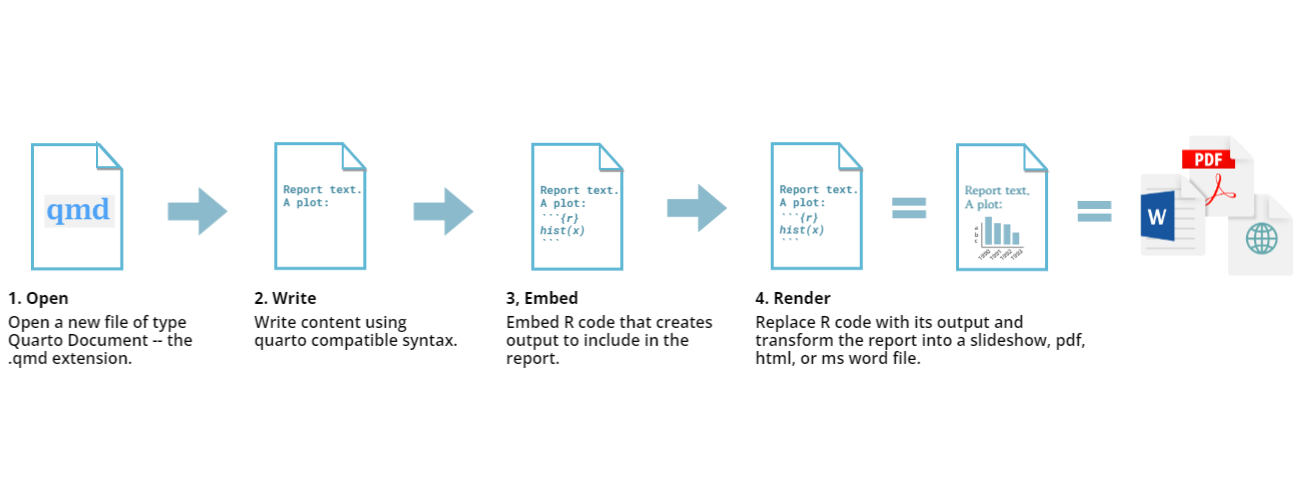
We don’t have the time to go into the details of Quarto during this lesson, but recommend the “Introduction to Reproducible Publications with RStudio” incubator (in-development) lesson for more on this topic.
Recommended workflow
Dynamic documents like Quarto (or Rmarkdown, the predecessor to
Quarto) can actually be used to manage data analysis pipelines. But that
is not recommended because it doesn’t scale well and lacks the
sophisticated dependency tracking offered by targets.
Our suggested approach is to conduct the vast majority of data
analysis (in other words, the “heavy lifting”) in the
targets pipeline, then use the Quarto document to
summarize and plot the results.
Report on bill size in penguins
Continuing our penguin bill size analysis, let’s write a report evaluating each model.
To save time, the report is already available at https://github.com/joelnitta/penguins-targets.
Copy the raw
code from here and save it as a new file
penguin_report.qmd in your project folder (you may also be
able to right click in your browser and select “Save As”).
Then, add one more target to the pipeline using the
tar_quarto() function like this:
R
source("R/functions.R")
source("R/packages.R")

tar_plan(
  # Load raw data
  tar_file_read(
    penguins_data_raw,
    path_to_file("penguins_raw.csv"),
    read_csv(!!.x, show_col_types = FALSE)
  ),
  # Clean and group data
  tar_group_by(
    penguins_data,
    clean_penguin_data(penguins_data_raw),
    species
  ),
  # Get summary of combined model with all species together
  combined_summary = model_glance(penguins_data),
  # Get summary of one model per species
  tar_target(
    species_summary,
    model_glance(penguins_data),
    pattern = map(penguins_data)
  ),
  # Get predictions of combined model with all species together
  combined_predictions = model_augment(penguins_data),
  # Get predictions of one model per species
  tar_target(
    species_predictions,
    model_augment(penguins_data),
    pattern = map(penguins_data)
  ),
  # Generate report
  tar_quarto(
    penguin_report,
    path = "penguin_report.qmd",
    quiet = FALSE
  )
)
The function to generate the report is tar_quarto(),
from the tarchetypes package.
As you can see, the “heavy” analysis of running the models is done in
the workflow, then there is a single call to render the report at the
end with tar_quarto().
How does targets know when to render the report?
It is not immediately apparent just from this how
targets knows to generate the report at the end of
the workflow (recall that build order is not determined by the
order of how targets are written in the workflow, but rather by their
dependencies). penguin_report does not appear to depend on
any of the other targets, since they do not show up in the
tar_quarto() call.
How does this work?
The answer lies inside the
penguin_report.qmd file. Let’s look at the start of the
file:
MARKDOWN
---
title: "Simpson's Paradox in Palmer Penguins"
format:
  html:
    toc: true
execute:
  echo: false
---

```{r}
#| label: load
#| message: false
targets::tar_load(
  c(combined_summary,
    species_summary,
    combined_predictions,
    species_predictions
  )
)

library(tidyverse)
```

The goal of this analysis is to determine how bill length and depth are related in three species of penguins from Antarctica.
The lines in between --- and --- at the
very beginning are called the “YAML header”, and contain directions
about how to render the document.
The R code to be executed is specified by the lines between
```{r} and ```. This is called a “code chunk”,
since it is a portion of code interspersed within prose text.
Take a closer look at the R code chunk. Notice the use of
targets::tar_load(). Do you remember what that function
does? It loads the targets built during the workflow.
Now things should make a bit more sense: targets knows
that the report depends on the targets built during the workflow like
combined_summary and species_summary
because they are loaded in the report with
tar_load().
Generating dynamic content
The call to tar_load() at the start of
penguin_report.qmd is really the key to generating an
up-to-date report—once those are loaded from the workflow, we know that
they are in sync with the data, and can use them to produce “polished”
text and plots.
Challenge: Spot the dynamic contents
Read through penguin_report.qmd and try to find
instances where the targets built during the workflow
(combined_summary, etc.) are used to dynamically produce
text and plots.
In the code chunk labeled
results-stats, statistics from the models like R squared are extracted, then inserted into the text with in-line code like`r combined_r2`.There are two figures, one for the combined model and one for the separate models (code chunks labeled
fig-combined-plotandfig-separate-plot, respectively). These are built using the points predicted from the model incombined_predictionsandspecies_predictions.
You should also interactively run the code in
penguin_report.qmd to better understand what is going on,
starting with tar_load(). In fact, that is how this report
was written: the code was run in an interactive session, and saved to
the report as it was gradually tweaked to obtain the desired
results.
The best way to learn this approach to generating reports is to try it yourself.
So your final Challenge is to construct a targets
workflow using your own data and generate a report. Good luck!
-
tarchetypes::tar_quarto()is used to render Quarto documents - You should load targets within the Quarto document using
tar_load()andtar_read() - It is recommended to do heavy computations in the main targets workflow, and lighter formatting and plot generation in the Quarto document