Visualising and quantifying linear associations

Overview

Teaching: 10 min
Exercises: 10 min

Questions

• How can we visualise the linear association between two variables?

• How can we quantify the size of a linear association?

Objectives

• Explore whether two variables appear to be associated using a scatterplot.

• Calculate the size of a linear association between two variables using Pearson’s correlation.

In this episode we will learn how to check whether two variables are linearly associated. This will allow us to use one variable to predict the mean of another variable in the next episode, when an association exists.

Visually checking for a linear association

The first way to check for a linear association is by using a scatterplot. For example, below we create a scatterplot of adult Weight vs. Height. We subset our data (dat) for adult participants using filter(), after which we specify the x and y axes in ggplot() and make a scatterplot using geom_point(). Note that dat is loaded into the environment by following the instructions on the setup page.

dat %>%
  filter(Age > 17) %>%
  ggplot(aes(x = Height, y = Weight)) +
  geom_point()

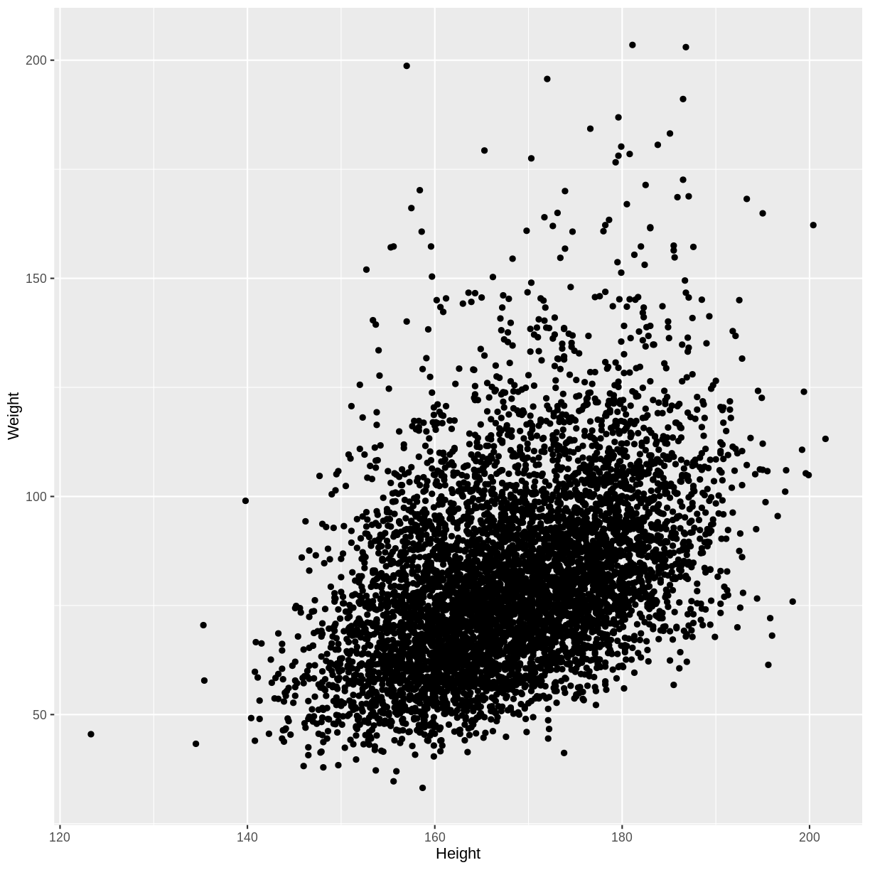
We see that on average, higher Weights are associated with higher Heights. This is an example of a positive linear association, as we see an increase along the y-axis as the values on the x-axis increase. The linear association suggests that we could use Heights to predict Weights.

In the exercise below you will explore examples of a negative linear association and an absence of a linear association.

Exercise

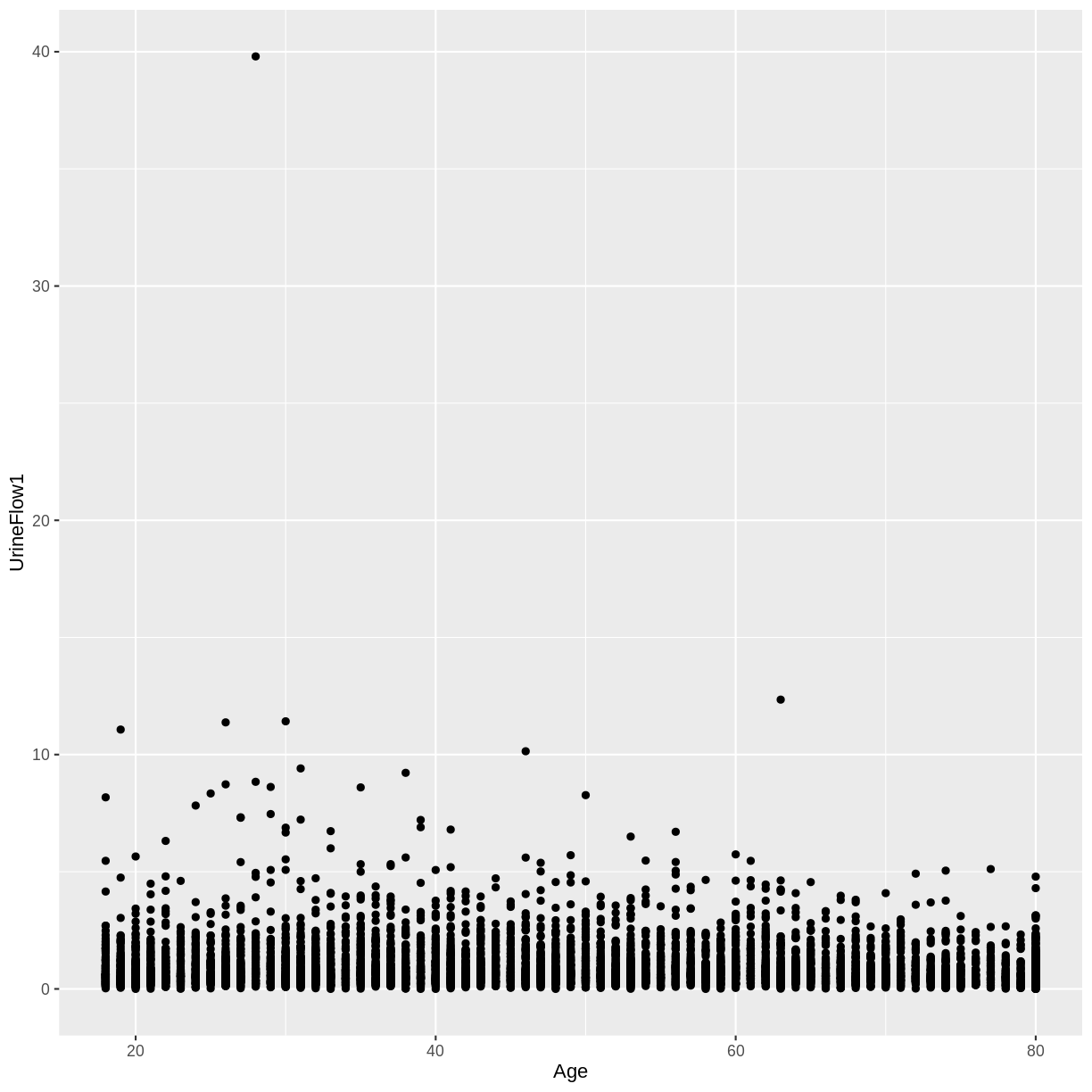
A) Create a scatterplot of urine flow (UrineFlow1) on the y-axis and age (Age) on the x-axis for adult participants. How would you describe the association between these variables?
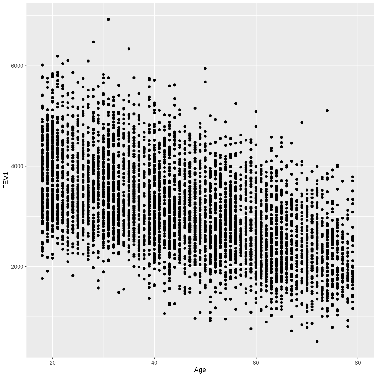
B) Create a scatterplot of FEV1 (FEV1) on the y-axis and age (Age) on the x-axis for adult participants. How would you describe the association between these variables?

Solution

A) There appears to be no linear association between urine flow and age.

dat %>%
  filter(Age > 17) %>%
  ggplot(aes(x = Age, y = UrineFlow1)) +
  geom_point() 

B) There appears to be a negative linear association between FEV1 and age.

dat %>%
  filter(Age > 17) %>%
  ggplot(aes(x = Age, y = FEV1)) +
  geom_point() 

Quantifying the size of a linear association

We can quantify the magnitude of a linear association using Pearson’s correlation coefficient. This metric ranges from -1 to 1.

• A value of -1 indicates a perfect negative linear association.
• A value of 1 indicates a perfect positive linear association.
• A value of 0 indicates absence of a linear association.

Let’s see these in practice by calculating the correlation coefficient for the associations that we explored above. To calculate the correlation coefficient between Weight and Height, we again select adult participants using filter(). Then, we calculate the correlation using the summarise() function. The correlation is given by the cor() function, where use = "complete.obs" ensures that participants for whom Weight or Height data is missing are ignored.

dat %>%
  filter(Age > 17) %>%
  summarise(correlation = cor(Weight, Height, use = "complete.obs"))

  correlation
1   0.4296817

The correlation coefficient of 0.43 is in line with the positive linear association that we saw above.

Exercise

A) Calculate the correlation coefficient for urine flow (UrineFlow1) and age (Age) in adult participants. Does this agree with the scatterplot?

B) Calculate the correlation coefficient for FEV1 (FEV1) and age (Age) in adult participants. Does this agree with the scatterplot?

Solution

A) The correlation coefficient near 0 is in agreement with the scatterplot.

dat %>%
  filter(Age > 17) %>%
  summarise(correlation = cor(UrineFlow1, Age, use = "complete.obs"))

  correlation
1 -0.07972899

B) The correlation coefficient of -0.55 is in agreement with the scatterplot.

dat %>%
  filter(Age > 17) %>%
  summarise(correlation = cor(FEV1, Age, use = "complete.obs"))

  correlation
1  -0.5487635

Key Points

• Scatterplots allow us to visually check the linear association between two variables.

• Pearson’s correlation coefficient allows us to quantify the size of a linear association.