Estimating the mean, variance and standard deviation

Overview

Teaching: 15 min
Exercises: 20 min

Questions

• How are the mean, variance and standard deviation calculated and interpreted?

Objectives

• Estimate the mean, variance and standard deviation of a variable through simulation.

Often when doing statistics, we have a variable of interest, for which we want to estimate particular properties. A variable will follow a distribution, which shows what values a variable can take and how likely these are to occur. In this episode we will learn to estimate and interpret the mean, variance and standard deviation of a variable’s distribution. These values allow us to estimate the average of a variable in the population and the variation around that average.

Before discussing the definitions of these values, let’s look at an example. The heights of people of the female sex in the US approximately follow a distribution with a mean of 162 cm and a standard deviation of 6.89 cm. The distribution is shown below. Values on the x-axis with a greater density on the y-axis have a higher chance of occurring. Under this distribution, a height of 162 cm would be most likely to occur, while a height of 140 cm would be very unlikely to occur.

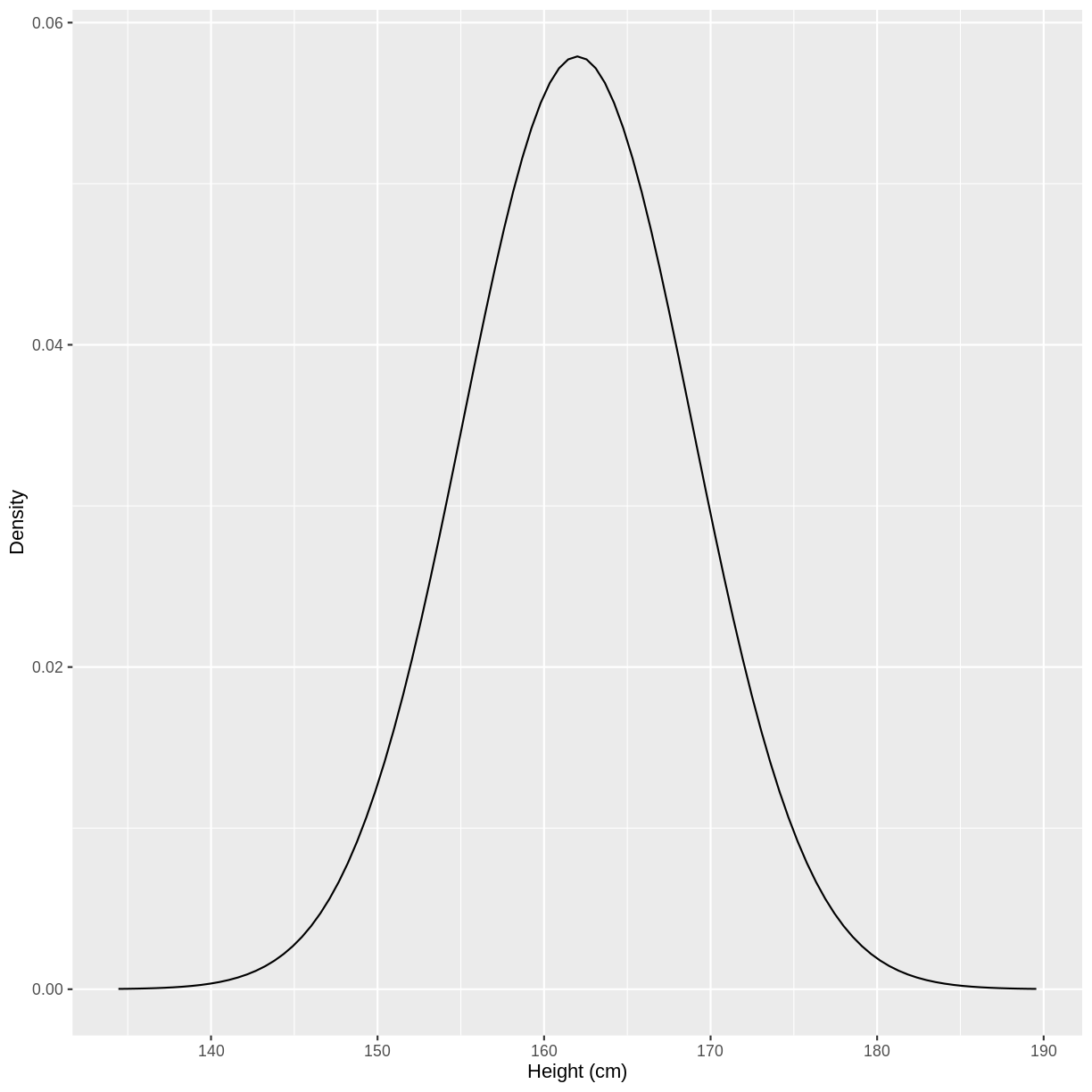
You may recognise the shape of the above distribution. It is an example of a normal distribution.

Let’s say that we sampled 1000 observations of female height through a survey. We can refer to these observations as $y_i$, with $i = 1, \dots, 1000$. The distribution of female heights has a few properties of interest, which we can estimate using our sample.

The mean

The population mean is the average of all the values that make up a distribution. In the case of female heights in the US, we will assume that the the population mean is 162 cm. Under this assumption, the average height of a US female is 162 cm.

After obtaining our sample of 1000 observations from the population, we may be interested in the sample mean. We expect our sample mean to equal the population mean, with a sufficiently large sample. The sample mean is expressed as $\bar{y}$:

where $n = 1000$.

The variance

The variance is the average squared difference between values in the distribution and the mean of the distribution. This is a mouthful, so it is useful to look at the equation of variance.

Here we will look at the sample variance, expressed as $s_{y}^2$:

Breaking this down, we see that the sample variance is calculated using:

• $y_{i} - \bar{y}$, i.e. the difference between an observed height and the sample mean height.
• $(y_{i} - \bar{y})^2$, i.e. the squared difference between an observed height and the sample mean height.
• $\frac{1}{n-1} \sum_{i=1}^n (y_i - \bar{y})^2 $, i.e. the mean of this squared difference. Note that we divide by $n-1$ rather than $n$, which is known as a bias correction. This allows us to estimate the population variance more accurately.

Why are we interested in this value? We are mainly interested in the variance because it allows us to calculate the standard deviation, which can be interpreted on the original scale. Let’s look at this below.

The standard deviation

The standard deviation of a distribution is the square root of the variance. The standard deviation is interpreted as a measure of the difference between values in the distribution and the mean of the distribution. A higher standard deviation indicates that the spread around the mean is greater. There is no “good” or “bad” standard deviation - its purpose is to give us an idea of the spread of observations in the population.

After obtaining our sample of 1000 observations from the population, we may be interested in the sample standard deviation. We expect our sample standard deviation to equal the population standard deviation, with a sufficiently large sample. The sample standard deviation is expressed as $s_y$:

Estimating the mean, variance and standard deviation through simulation

Another route to understanding the mean, variance and standard deviation is through simulation. This is the process of sampling data from a distribution using R. This is akin to collecting observations in the real world, where obervations come from an underlying distribution.

For example, we can sample 1000 observations from the distribution of female heights in the US using rnorm(). We store these values in a tibble, with the column named heights.

sample <- tibble(heights = rnorm(1000, mean = 162, sd = 6.89))

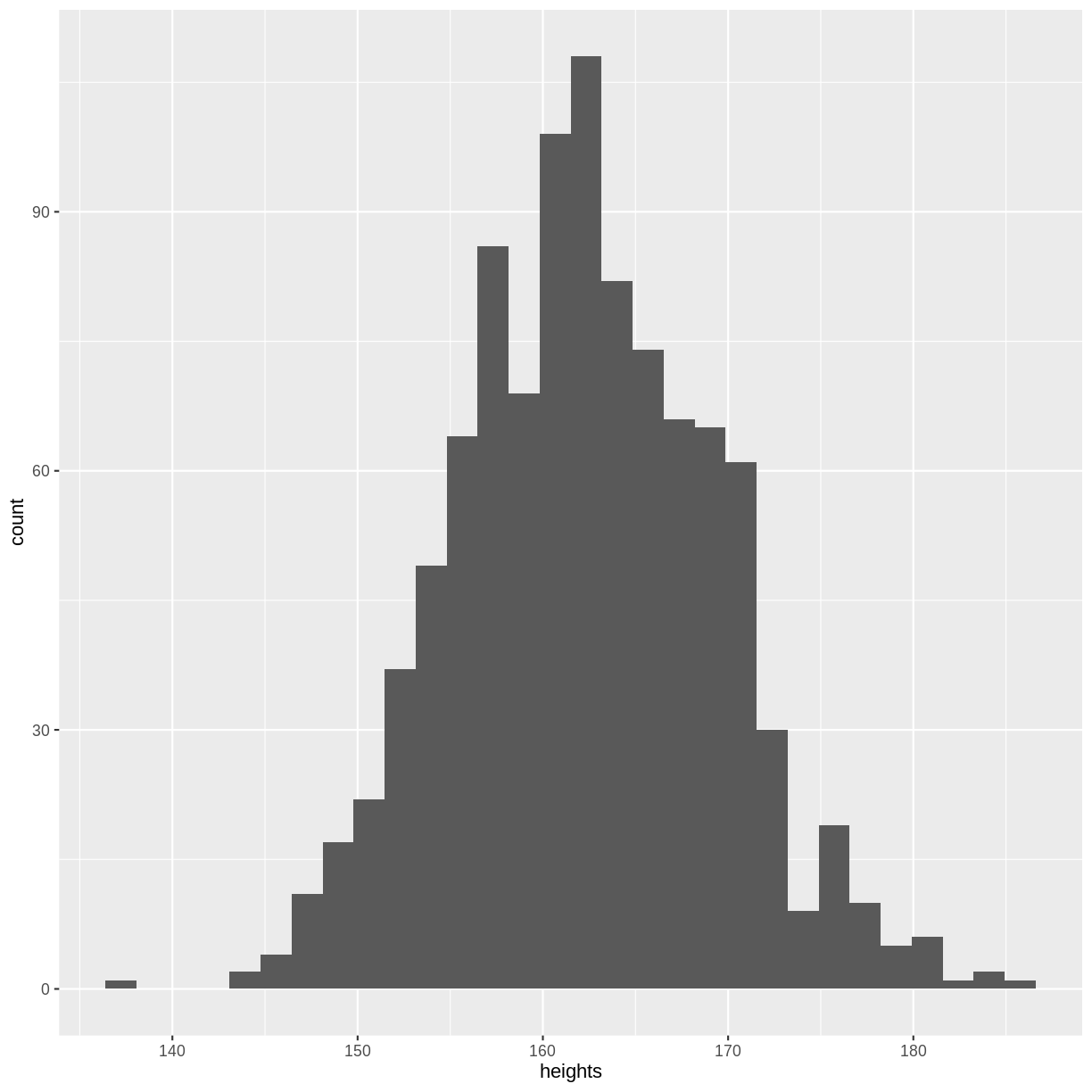
Before calculating the mean, variance and standard deviation, let’s create a histogram of our sample. Although not a perfect representation, our histogram looks quite similar to the distribution shown at the start of this episode. Your plot will differ slightly from the histogram shown below, as rnorm() obtained a random sample. If you create a new sample and run the ggplot() code again, the histogram will differ slightly again. Every sample contains 1000 new observations from the same distribution, akin to running an experiment where we collect 1000 observations.

ggplot(sample, aes(x = heights)) +
  geom_histogram()

We can calculate sample mean using mean(). This value lies close to the population mean of 162 cm. Here we see that the sample mean approximately equals the population mean with a sufficiently large sample.

meanHeight <- mean(sample$heights)
meanHeight

[1] 162.2838

We can also calculate the variance as the mean of the squared differences between our sampled observations and the sample mean, where sum() sums the squared differences and we divide by $n-1 = 999$:

varHeight <- (1/999) * sum( (sample$heights - meanHeight)^2 ) 
varHeight

[1] 49.26087

Finally, we calculate the sample standard deviation as the square root of the sample variance. The square root is obtained using sqrt(). Recall that we calculate the standard deviation to have a measure of spread in our distribution, in the same units as our original data (in this case, mmHg).

sdHeight <- sqrt(varHeight)
sdHeight

[1] 7.018609

Exercise

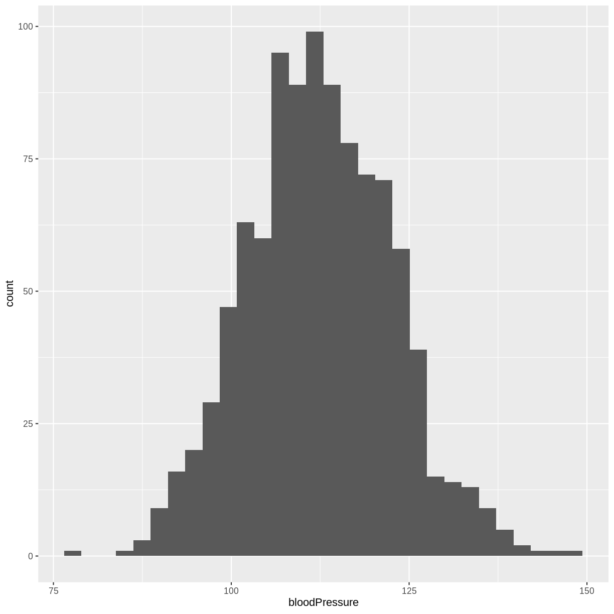
The normal distribution of systolic blood pressure has a mean of 112 mmHg and a standard deviation of 10 mmHg. The distribution looks as follows:

A) Sample one thousand observations from this distribution. Then, create a histogram of your sample.
B) Calculate the average systolic blood pressure in your sample. Does this value correspond to the population mean?
C) Calculate the variance of your sample.
D) Calculate the standard deviation of your sample. How is the standard deviation interpreted here?

Solution

Throughout this solution, your results will differ slightly from the ones shown below. This is a consequence of rnorm() drawing random samples. If you are completing this episode in a workshop setting, ask your neighbour to compare results! If you are working through this episode independently, try running your code again to see how the results differ.

A) We obtain 1000 observations from the systolic blood pressure distribution using rnorm(). We store these values in an object named sample. We then create a histogram using geom_histogram().

sample <- tibble(bloodPressure = rnorm(1000, mean = 112, sd = 10))

ggplot(sample, aes(x = bloodPressure)) +
  geom_histogram()

B) We can then calculate the average systolic blood pressure in our sample using mean(). The mean of our sample lies closely to the mean of the original distribution.

meanBP <- mean(sample$bloodPressure)
meanBP

[1] 112.4119

C) The variance equals the average of the squared differences between the mean of the distribution and the observed values. This can be calculated as follows:

varBP <- (1/999) * sum( (sample$bloodPressure - meanBP)^2 )
varBP

[1] 103.768

D) The standard deviation equals the square root of the variance. It is interpreted as a measure of the spread of sampled systolic blood pressure values and the mean systolic blood pressure. The square root can be calculated using sqrt().

sdBP <- sqrt(varBP)
sdBP

[1] 10.18666

Key Points

• The mean is the average value. The population has a population mean, while we estimate a sample mean from our sample.

• The sample variance is the average of the squared differences between values in our sample and the mean of our sample.

• The standard deviation is the square root of the variance. It measures the spread of observations around the mean, in units of the original data.