Estimating the variation around the mean: standard errors and confidence intervals

Overview

Teaching: 20 min
Exercises: 40 min

Questions

• What are the definitions of the standard error and the 95% confidence interval?

• How is the 95% confidence interval interpreted in practice?

Objectives

• Explore the difference between a population parameter and sample estimates by simulating data from a normal distribution.

• Define the 95% confidence interval by simulating data from a normal distribution.

In the previous episode, we obtained an estimate of the mean by simulating from a normal distribution. This simulation was akin to obtaining one sample in the real world. We learned that as is the case in the real world, every sample will differ from the next sample slightly.

In this episode, we will learn how to estimate the variation in the mean estimate. This will tell us how far we can expect the population mean to lie from our sample mean. We will also visualise the variation in the estimate of the mean, when we simulate many times from the same distribution. This will allow us to understand the meaning of the 95% confidence interval.

The standard error of the mean

In the previous episode, we learned that the standard deviation is a measure of the expected difference between a value in the distribution and the mean of the distribution. In this episode we will work with a related quantity, called the standard error of the mean (referred to hereafter as the standard error). The standard error quantifies the spread of sample means around the population mean.

For example, let’s say we collected 1000 observations of female heights in the US, to estimate the mean height. The standard error of this estimate in this case is 0.22 cm.

The standard error is calculated using the standard deviation and the sample size:

Therefore, for our female heights sample, the standard error was calculated as $\text{se}(y) = 6.89 / \sqrt{1000} \approx 0.22$ cm.

Notice that with greater $n$, the standard error will be smaller. This makes intuitive sense: with greater sample sizes come more precise estimates of the mean.

One of the reasons we calculate the standard error is that it allows us to calculate the 95% confidence interval, as we will do in the next section.

The 95% confidence interval

We use the standard error to calculate the 95% confidence interval. This interval equals, for large samples:

i.e. the mean +/- 1.96 times the standard error.

The definition of the 95% confidence interval is a bit convoluted:

95% of 95% confidence intervals are expected to contain the true population mean.

Imagine we were to obtain 100 samples of female heights in the US, with each sample containing 1000 observations. For each sample, we would calculate a mean and a 95% confidence interval. By the definition of the interval, we would expect approximately 95 of the intervals to contain the true mean of 162 cm. In other words, we would expect approximately 5 of our samples to give confidence intervals that do not contain the true mean of 162 cm.

What does this mean in practice? When we calculate a 95% confidence interval, we are fairly confident that it will contain the true population mean, but we cannot know for sure.

Let’s take a look at how we can calculate the 95% confidence interval in R. First, we sample 1000 observations of female heights and calculate the sample mean, as in the previous episode. Then, we calculate the standard error as the standard deviation divided by the square root of the sample size. Note the use of the sd() function, which returns the standard deviation (rather than the manual calculation used in the previous episode). Finally, the 95% confidence interval is given by the mean +/- 1.96 times the standard error. Note that your CI will differ slightly from the one shown below, as rnorm() obtains random samples.

sample <- tibble(heights = rnorm(1000, mean = 162, sd = 6.89))

meanHeight <- mean(sample$heights)

seHeight <- sd(sample$heights)/sqrt(1000)

CI <- c(meanHeight - 1.96 * seHeight, meanHeight + 1.96 * seHeight)
CI

[1] 161.7944 162.6394

The confidence interval shown above has a lower bound of 161.7898 and an upper bound of 162.6439. In this instance, we have obtained a 95% confidence interval that captures the population mean of 162. The confidence interval that you obtain may not capture the population mean of 162. It would then be part of the 5% of 95% confidence intervals that do not capture the population mean.

Exercise

A) Given the distribution of systolic blood pressure, with a population mean of 112 mmHg and a population standard deviation of 10 mmHg, obtain a random sample of 2000 observations.
B) Estimate the sample mean systolic blood pressure and provide a 95% confidence interval for this estimate. How do we interpret this interval?

Solution

Throughout this solution, your results will differ slightly from the ones shown below. This is a consequence of rnorm() drawing random samples. If you are completing this episode in a workshop setting, ask your neighbour to compare results! If you are working through this episode independently, try running your code again to see how the results differ.

A)

sample <- tibble(bloodPressure = rnorm(2000, mean = 112, sd = 10))

B)

meanBP <- mean(sample$bloodPressure)
seBP <- sd(sample$bloodPressure)/sqrt(2000)

CI <- c(meanBP - 1.96 * seBP, meanBP + 1.96 * seBP)
CI

[1] 111.3997 112.2691

The confidence interval has lower bound 111.4 and upper bound 112.27. The interval captures the population mean of 112 and therefore belongs to the 95% of 95% CIs that do capture the population mean. If your CI does not cover 112, then your CI belongs to the 5% of 95% CIs that do not capture the population mean.

Simulating 95% confidence intervals

In the previous section we learned that 95% of 95% confidence intervals are expected to contain the population mean. Let’s see this in action, by simulating 100 data sets of 1000 female heights.

First, we create a tibble for our means and confidence intervals. We name this tibble means and create empty columns for the sample IDs, mean heights, standard errors, the lower bound of the confidence intervals and the upper bound of the confidence intervals.

means <- tibble(sampleID = numeric(),
               meanHeight = numeric(),
               seHeight = numeric(),
               lower_CI = numeric(),
               upper_CI = numeric())

We simulate the Heights data using a for loop. This gives us 100 iterations, in which samples are drawn using rnorm(). For each sample, we add a row to our means tibble using add_row(). We include an ID for the sample, the mean Height, the standard error and the bounds of the 95% confidence interval.

for(i in 1:100){
 sample_heights <- rnorm(1000, mean = 162, sd = 6.89)
 
 means <- means %>%
   add_row(sampleID = i,
           meanHeight = mean(sample_heights),
           seHeight = sd(sample_heights)/sqrt(1000),
           lower_CI = meanHeight - 1.96 * seHeight,
           upper_CI = meanHeight + 1.96 * seHeight)
}

Finally, we add a column to our means tibble that indicates whether a confidence interval contains the true population mean of 162 cm.

means <- means %>%
 mutate(capture = ifelse((lower_CI < 162 & upper_CI > 162),
                           "Yes", "No"))

Now we are ready to plot our means and confidence intervals. The following code plots the mean estimates along the x-axis using geom_point(), with sample IDs along the y-axis. Confidence intervals are added to these points using geom_errorbar(). The population mean is displayed as a dashed line using geom_vline(). Finally, confidence intervals are coloured by whether they capture the true population mean.

ggplot(means, aes(x = meanHeight, y = sampleID, colour = capture)) +
 geom_point() +
 geom_errorbar(aes(xmin = lower_CI, xmax = upper_CI, colour = capture)) +
 geom_vline(xintercept = 162, linetype = "dashed") +
 scale_color_manual("Population mean captured",
                    values = c("magenta", "black"))

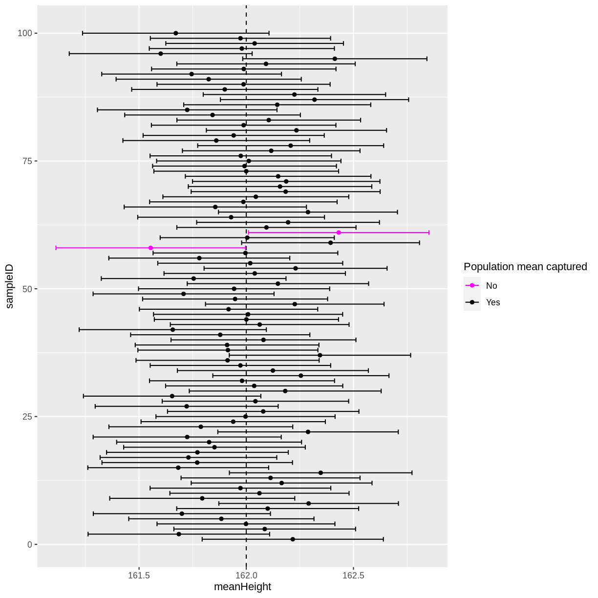
In this instance, 2 out of 100 95% confidence intervals did not capture the population mean. If you run the above code multiple times, you will discover that there is variation in the number of confidence intervals that capture the population mean. On average, 5 out of 100 95% confidence intervals will not capture the population mean.

Exercise

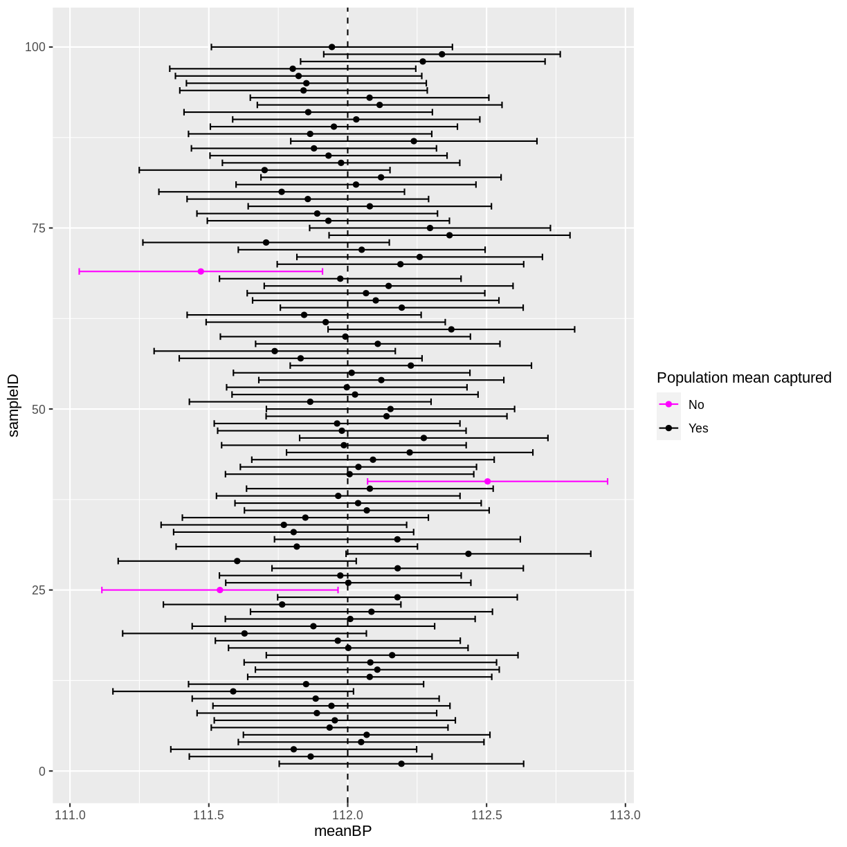
A) Given the distribution of systolic blood pressure, with a mean of 112 mmHg and a standard deviation of 10 mmHg, simulate 100 data sets of 2000 observations each. For each sample, store the sample ID, mean systolic blood pressure, the standard error and the 95% confidence interval in a tibble.
B) Create an extra column in the tibble, indicating for each confidence interval whether the original mean of 112 mmHg was captured.
C) Plot the mean values and their 95% confidence intervals. Add a line to show the population mean. How many of your 95% confidence intervals do not contain the true population mean of 112 mmHg?
D) Increase or decrease the number of observations sampled per data set in part A. Then, run through parts A, B and C again. What happened to the width of the confidence intervals? Did the interpretation of the confidence intervals change in any way?

Solution

Throughout this solution, your results will differ slightly from the ones shown below. This is a consequence of rnorm() drawing random samples. If you are completing this episode in a workshop setting, ask your neighbour to compare results! If you are working through this episode independently, try running your code again to see how the results differ.

A)

means <- tibble(sampleID = numeric(),
                meanBP = numeric(),
                seBP = numeric(),
                lower_CI = numeric(),
                upper_CI = numeric())


for(i in 1:100){
  
  sample_bp <- rnorm(2000, mean = 112, sd = 10)
  
  means <- means %>%
    add_row(sampleID = i,
            meanBP = mean(sample_bp),
            seBP = sd(sample_bp)/sqrt(2000),
            lower_CI = meanBP - 1.96 * seBP,
            upper_CI = meanBP + 1.96 * seBP)
}

B)

means <- means %>%
  mutate(capture = ifelse((lower_CI < 112 & upper_CI > 112),
                            "Yes", "No"))

C) In this instance, three 95% confidence intervals did not contain the true population mean. Since rnorm() draws random samples, you may have more or less 95% confidence intervals that capture the true population mean. On average, we 5 out of 100 95% confidence intervals will fail to capture the population mean.

ggplot(means, aes(x = meanBP, y = sampleID, colour = capture)) +
  geom_point() +
  geom_errorbar(aes(xmin = lower_CI, xmax = upper_CI, colour = capture)) +
  geom_vline(xintercept = 112, linetype = "dashed") +
  scale_color_manual("Population mean captured",
                     values = c("magenta", "black"))

D) Increasing the number of observations per data set decreases the width of confidence intervals. Decreasing the number of observations per data set has the opposite effect. However, the interpretation of the confidence intervals remains the same: we still have on average 5 out of 100 intervals that do not capture the true population mean.

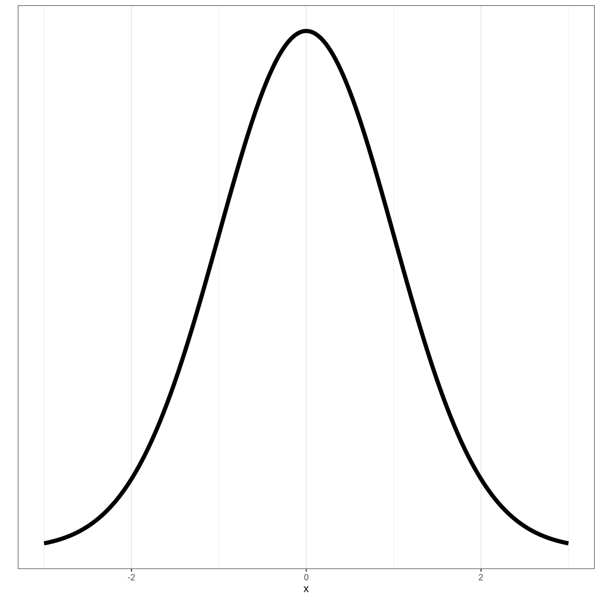
Why is the confidence interval calculated with 1.96?

To understand where the 1.96 mulitplier comes from, we need to look at the standard normal distribution. The standard normal distribution is a normal distribution with a mean of 0 and a standard deviation of 1:

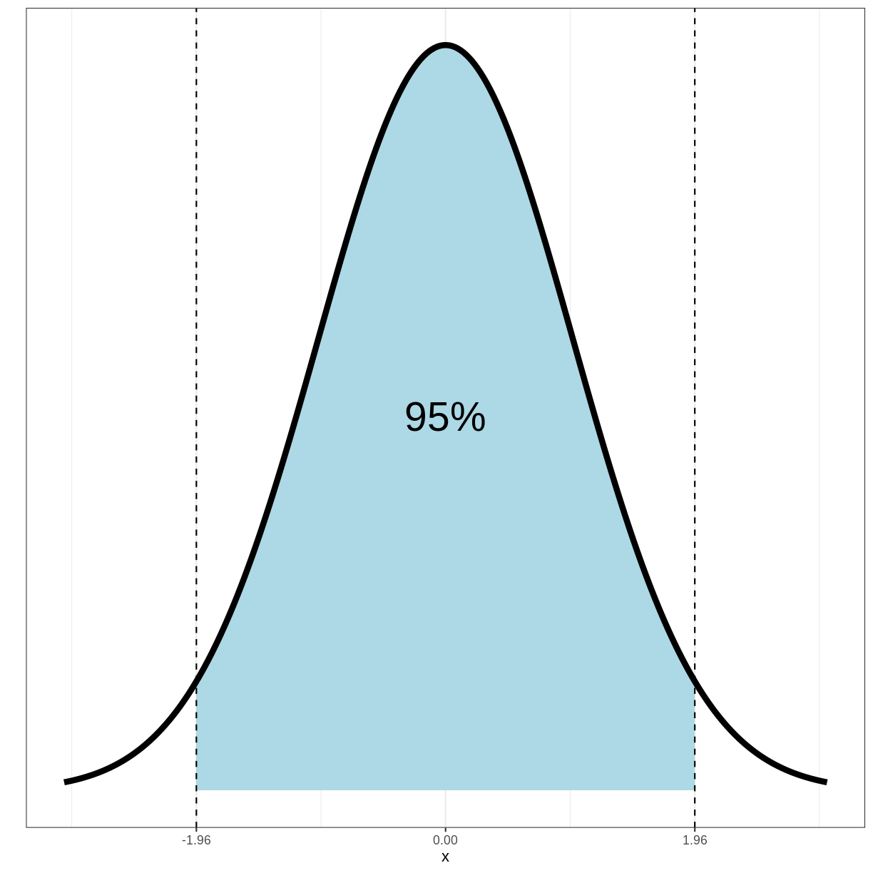
Importantly, 95% of the density of this distribution falls within the range of -1.96 and 1.96:

It can be shown that for a sample mean $\bar{X}$, coming from a normal sampling distribution, $Z$ follows a standard normal distribution:

\[Z = \frac{\bar{X}-\mu}{\sigma / n}\]

Here, $\mu$ is the population mean, $\sigma$ is the population standard deviation and $n$ is the sample size.

Since 95% of the density of the standard normal distribution falls between -1.96 and 1.96, the following holds:

\[Pr(-1.96 < Z < 1.96) = 0.95\]

Filling in $Z$ gives us:

\[Pr(-1.96 < \frac{\bar{X}-\mu}{\sigma / n} < 1.96) = 0.95\]

Which can be derived to:

\[Pr(\bar{X} -1.96 \frac{\sigma}{n} < \mu < \bar{X} + 1.96 \frac{\sigma}{n}) = 0.95\]

Since 95% of 95% confidence intervals will contain the true population mean $\mu$, the 95% confidence interval is given by $\bar{X} \pm 1.96 \times \frac{\sigma}{n}$, i.e. $\bar{X} \pm 1.96 \times se(X)$

Key Points

• Sample means are expected to differ from the population mean. We quantify the spread of estimated means around the population mean using the standard error.

• 95% of 95% confidence intervals are expected to capture the population mean. In practice, this means we are fairly confident that a 95% confidence interval will contain the population mean, but we do not know for sure.