Introduction
Overview
Teaching: 15 min
Exercises: 10 minQuestions
What are common use cases for timeseries analysis?
Objectives
Read and plot timeseries data using Python Pandas.
Group data and generate descriptive statistics.
Resample timeseries data using datetime indexing in Pandas.
Introducing time series
We regularly encounter time series data in our daily lives. Examples are abundant and include stock prices, daily rates of infection during the COVID-19 pandemic, gas and electricity use as described in our utility bills, and data points from our fitness tracking devices. Any type of observation for which data are collected at specific intervals can be represented as a time series.
Time series data may be analyzed for multiple purposes, including
- Identifying trends.
- Making forecasts.
- Fraud and anomaly detection.
This series of lessons is intended as an introduction to key concepts in the analysis and visualization of time series data. Additional lessons in this series will introduce concepts and methods for making forecasts and classifying time series for different purposes.
Challenge: Time series in our daily lives
Above, we provided examples of information that is best represented using time series, for example daily prices of stocks.
What are some other examples of information that is collected consecutively or at specific intervals? Think of an example and reflect on the following questions:
- Are observations recorded at specific times?
- Are observations recorded at regular intervals?
- What types of trends would you expect to see in the data?
Time series analysis using Python
Several Python libraries have been developed which can be used to support analysis of trends, forecasting, and classification of time series data. A non-exhaustive list of libraries includes:
pandas()statistics()scikitlearn()tensorflow()
This lesson is focused on Pandas, which provides many useful features for inspecting large datasets, as well as resampling time series data to quickly calculate and plot statistics and moving averages.
Key Points
Pandas is a Python library that operates efficiently against large datasets.
Datetime indexing with Pandas enables resampling of timeseries data using different time steps.
Reading Data Files with Python
Overview
Teaching: 45 min
Exercises: 20 minQuestions
How can we manipulate tabular data files in Python?
Objectives
Read tabular data from a file into Pandas.
Change the structure of a dataframe.
Combine multiple files into a single dataset.
Our data have been stored in one CSV file per smart meter, in which the data include all of the meter readings taken from that meter during the period of study. Readings are taken every 15 minutes, for a total of 96 readings per day.
The structure of the data has not been altered from the source data. Each CSV file contains the following fields:
- METER_FID: The identification number of the meter for which the data were recorded.
- START_READ: The meter reading at 00:15 (12:15 AM) of the date specified in the INTERVAL_TIME field. Note that this value is the same for each reading taken during a day, and is the same as the END_READ value of the previous day.
- END_READ: The actual value of the meter after the final interval of the date specified in the INTERVAL_TIME field, representing the total amount of power consumed during the whole day. This value becomes the value of the START_READ field for the next day.
- INTERVAL_TIME: The time at which a meter reading was taken. Readings are taken every 15 minutes, with the first reading for a day taken at 00:15 (12:15 AM) and representing power usage since 00:00 (12:00 AM) of the same day.
- INTERVAL_READ: The amount of power consumed between readings. The sum of readings between 00:15 of a given day and 00:00 of the following day should be equal (to two decimal places) to the difference between the END_READ and START_READ values for that day.
In order to inspect and analyze the data for each meter, we could read and work with each file independently. However, as we may also want to compare statistics or trends across multiple meters, it can be more practical to combine or concatenate the data from multiple meters into a single dataset. Having done that, we can group the data by meter, date, or other variables of interest. The Pandas library for Python allows us to do just this.
Libraries
When you launch a Python environment, it opens with a set of default libraries loaded. These libraries provide access to a default set of functions, including commonly used functions like print() and help(). Libraries can be used to extend the functionality of the environment beyond the default. Here, we are going to import the pandas and glob libraries to add functionality to our environment. Specifically, pandas is a library that provides methods for indexing and manipulating large datasets. The glob library allows us to quickly create lists of files based on patterns in filenames.
import pandas as pd
import glob
Reading files
Creating a list of filenames that we want to read is a common way of iterating over files in Python. We use glob to create the list, though for now we will only read the first file in the list.
file_list = glob.glob('../data/*.csv')
print(file_list)
Lists may or may not be sorted in Python. That is, our files may appear in any order in the list. We can sort the files by name before reading the first file.
file_list = sorted(file_list)
data = pd.read_csv(file_list[0])
Inspecting the data
The data is assigned to the variable data, which is an object.
Get information about data as an object, and also information about the data.
# Find the data type of the 'data' object

print(type(data))
<class 'pandas.core.frame.DataFrame'>
We can get information about the data by requesting its attributes or using functions.
Use the shape attribute to see the size in rows and columns.
print(data.shape)
(105012, 5)
Use the dtypes attribute to see the data types of all columns in the dataset.
print(data.dtypes)
INTERVAL_TIME     object
METER_FID          int64
START_READ       float64
END_READ         float64
INTERVAL_READ    float64
dtype: object
We can limit the above to a single column.
print(data.START_READ.dtypes)
dtype('float64')
shape and dtypes are two examples of attributes.
We can also use functions or methods to see information about the dataframe.
The info() function outputs structural information about the data.
print(data.info())
<class 'pandas.core.frame.DataFrame'>
RangeIndex: 105012 entries, 0 to 105011
Data columns (total 5 columns):
 #   Column         Non-Null Count   Dtype
---  ------         --------------   -----
 0   INTERVAL_TIME  105012 non-null  object
 1   METER_FID      105012 non-null  int64
 2   START_READ     105012 non-null  float64
 3   END_READ       105012 non-null  float64
 4   INTERVAL_READ  105012 non-null  float64
dtypes: float64(3), int64(1), object(1)
memory usage: 4.0+ MB
None
Note that info() prints out all of the information we got from the type() function and the shape and dtypes attributes.
We can also inspect some rows of data. Since the table is large - over 100,000 rows - we may only want to look at the first few or the last few rows. To do this, we can use the head() and tail() functions, respectively.
print(data.head())
         INTERVAL_TIME  METER_FID  START_READ   END_READ  INTERVAL_READ
0  2017-01-01 00:00:00        285   14951.787  14968.082         0.0744
1  2017-01-01 00:15:00        285   14968.082  14979.831         0.0762
2  2017-01-01 00:30:00        285   14968.082  14979.831         0.1050
3  2017-01-01 00:45:00        285   14968.082  14979.831         0.0636
4  2017-01-01 01:00:00        285   14968.082  14979.831         0.0870
print(data.tail())
              INTERVAL_TIME  METER_FID  START_READ   END_READ  INTERVAL_READ
105007  2019-12-31 22:45:00        285   28358.546  28397.749         0.4944
105008  2019-12-31 23:00:00        285   28358.546  28397.749         0.4974
105009  2019-12-31 23:15:00        285   28358.546  28397.749         0.4422
105010  2019-12-31 23:30:00        285   28358.546  28397.749         0.4212
105011  2019-12-31 23:45:00        285   28358.546  28397.749         0.3816
So far we have called all of the functions using default arugments. For example, by default head() and tail() will
print the first or last five rows. If we want to view more (or fewer) rows, we can pass the number of rows as an argument. If for example
we wanted to see the first ten rows of data, we would pass that number as the argument:
print(data.head(10))
         INTERVAL_TIME  METER_FID  START_READ   END_READ  INTERVAL_READ
0  2017-01-01 00:00:00        285   14951.787  14968.082         0.0744
1  2017-01-01 00:15:00        285   14968.082  14979.831         0.0762
2  2017-01-01 00:30:00        285   14968.082  14979.831         0.1050
3  2017-01-01 00:45:00        285   14968.082  14979.831         0.0636
4  2017-01-01 01:00:00        285   14968.082  14979.831         0.0870
5  2017-01-01 01:15:00        285   14968.082  14979.831         0.0858
6  2017-01-01 01:30:00        285   14968.082  14979.831         0.0750
7  2017-01-01 01:45:00        285   14968.082  14979.831         0.0816
8  2017-01-01 02:00:00        285   14968.082  14979.831         0.0966
9  2017-01-01 02:15:00        285   14968.082  14979.831         0.0720
Challenge: Know Your Data
Which of the following commands will output the data type of the ‘INTERVAL_TIME' column in our ‘data’ dataframe?
A. print(type(INTERVAL_TIME))
B. print(data.info())
C. print(data.INTERVAL_TIME.dtypes)
D. print(INTERVAL_TIME.dtypes)
Solution
B and C will both work. Option B prints the dtypes
for the whole dataframe. Option C prints the dtype
for the INTERVAL_TIME column.
Challenge: Drilling Down
We have seen how we can use dot notation to get the ‘dtypes’ information for a single column:
print(data.START_READ.dtypes)Dot notation can be used in function calls, too. Which of the following commands would we use to view the first 20 rows of data from the START_READ column:
A. print(data.START_READ.head())
B. print(data.START_READ.info())
C. print(data.head(20).START_READ)
D. print(data.START_READ.head(20))
Solution
Options C and D print out the first 20 rows of data
from the START_READ column.
Modifying data frames - adding columns
If we inspect the first five rows of the INTERVAL_TIME column, we see that dates are provided in a long format.
print(data.INTERVAL_TIME.head())
0    2017-01-01 00:00:00
1    2017-01-01 00:15:00
2    2017-01-01 00:30:00
3    2017-01-01 00:45:00
4    2017-01-01 01:00:00
Name: INTERVAL_TIME, dtype: object
Note as well that the data type (dtype) is given as object, even though datetime is a data type recognized by Pandas. In order to use date information in analyses, we can convert the data in the INTERVAL_TIME column into a recognized date format. In a later episode, we will look at ways we can manipulate datetime information by creating a datetime index. For now we will begin by exploring some of Pandas datetime methods without reindexing the data.
We can change the data type of the “INTERVAL_TIME” column in place, but for a closer look at what is happening we will save the date data in a new column with the updated data type.
data["iso_date"] = pd.to_datetime(data["INTERVAL_TIME"], infer_datetime_format=True)
We can verify that the new column was added and that the data type of the new column is datetime using the info() command.
print(data.info())
<class 'pandas.core.frame.DataFrame'>
RangeIndex: 105012 entries, 0 to 105011
Data columns (total 6 columns):
 #   Column         Non-Null Count   Dtype
---  ------         --------------   -----
 0   INTERVAL_TIME  105012 non-null  object
 1   METER_FID      105012 non-null  int64
 2   START_READ     105012 non-null  float64
 3   END_READ       105012 non-null  float64
 4   INTERVAL_READ  105012 non-null  float64
 5   iso_date       105012 non-null  datetime64[ns]
dtypes: datetime64[ns](1), float64(3), int64(1), object(1)
memory usage: 4.8+ MB
None
Note too that we are adding the new column but leaving the original date data intact.
Combining multiple files into a single dataframe
Now that we have read a single file into our Python environment and explored its structure a little, we want to develop a process to combine all of our data files into a single dataframe. We can do this using list comprehension to read the files in our file list and concatenate them into a single dataframe.
To do this, we will re-assign our data variable to include the complete, concatenated dataset. Note that it is a large dataset, with over 1,500,000 rows.
data = pd.concat([pd.read_csv(f) for f in file_list])
print(data.info())
<class 'pandas.core.frame.DataFrame'>
Int64Index: 1575180 entries, 0 to 105011
Data columns (total 5 columns):
 #   Column         Non-Null Count    Dtype
---  ------         --------------    -----
 0   INTERVAL_TIME  1575180 non-null  object
 1   METER_FID      1575180 non-null  int64
 2   START_READ     1575180 non-null  float64
 3   END_READ       1575180 non-null  float64
 4   INTERVAL_READ  1575180 non-null  float64
dtypes: float64(3), int64(1), object(1)
memory usage: 72.1+ MB
None
Let’s take a moment to unpack the line of code that creates the dataframe:
data = pd.concat([pd.read_csv(f) for f in file_list])
This line of code includes several statements that are evaluated in the following order:
- The for loop
for f in file_listis evaluated first. As denoted by the square brackets, this creates a list of dataframes by calling Pandas’read_csv()function on each of the files in the file_list variable that we created above. - The list of 15 dataframes is combined into a single dataframe using the
concat()function. This function takes as its default argument a list of dataframes that share the same structure, and combines them vertically into a single dataframe.
Now we can add the iso_date column using the same command as before:
data["iso_date"] = pd.to_datetime(data["INTERVAL_TIME"], infer_datetime_format=True)
print(data.info())
<class 'pandas.core.frame.DataFrame'>
Int64Index: 1575180 entries, 0 to 105011
Data columns (total 6 columns):
 #   Column         Non-Null Count    Dtype
---  ------         --------------    -----
 0   INTERVAL_TIME  1575180 non-null  object
 1   METER_FID      1575180 non-null  int64
 2   START_READ     1575180 non-null  float64
 3   END_READ       1575180 non-null  float64
 4   INTERVAL_READ  1575180 non-null  float64
 5   iso_date       1575180 non-null  datetime64[ns]
dtypes: datetime64[ns](1), float64(3), int64(1), object(1)
memory usage: 84.1+ MB
None
Challenge: Separating Dates into Columns
It can be useful in a variety of contexts to split date data into multiple columns, with one column for the year, one for the month, and another for the day. This can facilitate filtering or ordering by date in systems like SQLite, for example, that don’t by default have a date data type.
Given the lines of code below, put them in the correct order to read the data file “ladpu_smart_meter_data_01.csv” and split the “INTERVAL_TIME” column into three new columns for “year,” “month,” and “day.”
data["day"] = pd.to_datetime(data["INTERVAL_TIME"], infer_datetime_format=True).dt.day

data["year"] = pd.to_datetime(data["INTERVAL_TIME"], infer_datetime_format=True).dt.year

data = pd.read_csv("../data/ladpu_smart_meter_data_01.csv")

data["month"] = pd.to_datetime(data["INTERVAL_TIME"], infer_datetime_format=True).dt.month
Solution
data = pd.read_csv("../data/ladpu_smart_meter_data_01.csv")

data["year"] = pd.to_datetime(data["INTERVAL_TIME"], infer_datetime_format=True).dt.year

data["month"] = pd.to_datetime(data["INTERVAL_TIME"], infer_datetime_format=True).dt.month

data["day"] = pd.to_datetime(data["INTERVAL_TIME"], infer_datetime_format=True).dt.day
Key Points
PANDAS is a Python library designed to work with large datasets.
Use
concat()to concatenate tabular dataframes that have the same structure.
Subsetting Dataframes with PANDAS
Overview
Teaching: 30 min
Exercises: 15 minQuestions
How can we filter and subset data in Python?
Objectives
Understand how Pandas indexes data.
Subset dataframes using index positions and filtering criteria.
Pandas is designed to work with large datasets. Multiple indexing features allow for quick subsetting and filtering of data.
Rows and columns
The axes of a dataframe are the rows and columns. Both rows and column labels are indexed when a dataframe is created, such as when reading a CSV file into memory. This allows for quick selection of specific rows, columns, or cells, either through slicing or subsetting a dataframe by filtering values according to specific criteria.
It’s important to keep this terminology clear, because in addition to indexing rows and column labels, Pandas creates an index of row labels for every dataframe. This index can be specified when the dataframe is created, or alternatively Pandas will create an integer based index of row labels by default.
We can demonstrate this by reading a single file from our dataset. First, let’s load the libraries we will use for this episode.
import pandas as pd
import glob
Next we use the glob() function to create a list of files. Then we use the same process as before to read all of the files into a single large dataframe. We will also use the info() function to look at the structure of our dataframe.
file_list = glob.glob("../data/*.csv")
data = pd.concat([pd.read_csv(f) for f in file_list])
print(data.info())
<class 'pandas.core.frame.DataFrame'>
Int64Index: 1575180 entries, 0 to 105011
Data columns (total 5 columns):
 #   Column         Non-Null Count    Dtype
---  ------         --------------    -----
 0   INTERVAL_TIME  1575180 non-null  object
 1   METER_FID      1575180 non-null  int64
 2   START_READ     1575180 non-null  float64
 3   END_READ       1575180 non-null  float64
 4   INTERVAL_READ  1575180 non-null  float64
dtypes: float64(3), int64(1), object(1)
memory usage: 72.1+ MB
None
We can use the axes attribute to inspect the row and column indices. The output gives the row index first, and the column index second.
print(data.axes)
[Int64Index([     0,      1,      2,      3,      4,      5,      6,      7,
                 8,      9,
            ...
            105002, 105003, 105004, 105005, 105006, 105007, 105008, 105009,
            105010, 105011],
           dtype='int64', length=1575180), Index(['INTERVAL_TIME', 'METER_FID', 'START_READ', 'END_READ',
       'INTERVAL_READ'],
      dtype='object')]
The output above is a list, and the row index of our dataframe is the first object in the list:
[Int64Index([     0,      1,      2,      3,      4,      5,      6,      7,
                 8,      9,
            ...
            105002, 105003, 105004, 105005, 105006, 105007, 105008, 105009,
            105010, 105011],
           dtype='int64', length=1575180), Index(['INTERVAL_TIME', 'METER_FID', 'START_READ', 'END_READ',
       'INTERVAL_READ'],
      dtype='object')]
This indicates that our rows are indexed or labeled using incremented integers, beginning with the first row labeled 0 and the last row labeled 105011. Recall that Python uses zero-indexing, so the final value in the index should be understood as “up to but not including 105011.”
The final row index number may be surprising. The output of the info() function above indicates that our dataframe has 1,575,180 rows. But here the last row has an index number of 105011. Why is this?
When we created our dataframe, we did so by reading all of the files in our file list and concatenating them into a single dataframe. Each file was first read into its own dataframe before concatenation, which means that each of the 15 dataframe had its own row index beginning with 0 and stopping at whatever the last row index would be for that dataframe. When dataframes are concatenated, original row index numbers are preserved by default. Because of this, many thousands of row index numbers would have been common across datasets, resulting in duplicate row index numbers in the concatenated dataframe.
To make the most efficient use of Pandas in this case, we can reset the index of the dataframe. After resetting the index, we will check the axes attribute again.
data.reset_index(inplace=True, drop=True)
print(data.axes)
[RangeIndex(start=0, stop=1575180, step=1), Index(['index', 'INTERVAL_TIME', 'METER_FID', 'START_READ', 'END_READ',
       'INTERVAL_READ'],
      dtype='object')]
Note that this time the index is identified as a RangeIndex, rather than the Int64index that was output before. Instead of listing every integer index number, the range is given. This means that our rows are indexed or labeled using incremented integers, beginning with the first row labeled 0 and the last row labeled 1575810. Recall that Python uses zero-indexing, so the stop value in the RangeIndex should be understood as “up to but not including 1575180.” We can confirm this by referring to the output of the info() function above, which states that the dataframe index has 1575180 entries, labeled from 0 to 1575179.
The second object in the list output by printing the dataframe’s axes attribute is the column index. By default, the items in this index will be the column names, which can also be understood as the column axis labels:
Index(['INTERVAL_TIME', 'METER_FID', 'START_READ', 'END_READ',
       'INTERVAL_READ']
We can see the row labels using the head() function. Note that there is no column name for the row index. This is because there was no source column in our CSV file that the row labels refer to. We will update the attributes of the row index below.
print(data.head())
         INTERVAL_TIME  METER_FID  START_READ   END_READ  INTERVAL_READ
0  2017-01-01 00:00:00        285   14951.787  14968.082         0.0744
1  2017-01-01 00:15:00        285   14968.082  14979.831         0.0762
2  2017-01-01 00:30:00        285   14968.082  14979.831         0.1050
3  2017-01-01 00:45:00        285   14968.082  14979.831         0.0636
4  2017-01-01 01:00:00        285   14968.082  14979.831         0.0870
Selecting Specific Columns
If we want to select all of the values in a single column, we can use the column name.
print(data["INTERVAL_TIME"])
0          2017-01-01 00:00:00
1          2017-01-01 00:15:00
2          2017-01-01 00:30:00
3          2017-01-01 00:45:00
4          2017-01-01 01:00:00
                  ...
1575175    2019-12-31 22:45:00
1575176    2019-12-31 23:00:00
1575177    2019-12-31 23:15:00
1575178    2019-12-31 23:30:00
1575179    2019-12-31 23:45:00
Name: INTERVAL_TIME, Length: 1575180, dtype: object
In order to select multiple columns, we need to provide the column names as a list.
print(data[["METER_FID", "INTERVAL_TIME"]])
         METER_FID        INTERVAL_TIME
0              285  2017-01-01 00:00:00
1              285  2017-01-01 00:15:00
2              285  2017-01-01 00:30:00
3              285  2017-01-01 00:45:00
4              285  2017-01-01 01:00:00
...            ...                  ...
1575175       8078  2019-12-31 22:45:00
1575176       8078  2019-12-31 23:00:00
1575177       8078  2019-12-31 23:15:00
1575178       8078  2019-12-31 23:30:00
1575179       8078  2019-12-31 23:45:00
Note that all of our output includes row labels.
We can request attributes or perform operations on subsets.
print(data["INTERVAL_TIME"].shape)
(1575180,)
print(data["INTERVAL_READ"].sum())
365877.39449999994
Challenge: Find the Maximum Value of a Column
In addition to getting the sum of values from a a specific column, Pandas has functions for generating other statistics. These include
min()for the minimum value within a column andmax()for the maximum value.Which of the below lines of code would give us the maximum values of both the “START_READ” and “END_READ” columns?
A. print(data[START_READ, END_READ].max())
B. print(data["START_READ", "END_READ"].max())
C. print(data[[START_READ, END_READ]].max())
D. print(data[["START_READ", "END_READ"]].max())
Solution
Option D prints out the maximum value of the columns.
Challenge: Perform Operations on Specific Data Types
In addition to selecting columns by name, Pandas has a
select\_dtypes()method that lets us select columns of a specific data type.Which of the options below will print out the sum of each column with a
floatdata type?A. print(data.select_dtypes(float).sum()) B. print(data.select_dtypes([["START_READ", "END_READ", "INTERVAL_READ"]]).sum()) C. print(data[["START_READ", "END_READ", "INTERVAL_READ"]].sum()) D. print(data.sum(select_dtypes(float))Solution
Both A and C will output the correct result. However, option C requires us to already know that those columns have data of the correct data type.
Selecting Specific Rows
Subsets of rows of a Pandas dataframe can be selected different ways. The first two methods we’ll look at, .loc and .iloc indexing, have some subtle differences that are worth exploring.
.loc indexing will select rows with specific labels. Recall from earlier that when we read our CSV file into a dataframe, a row index was created which used integers as the label for each row. We can see information about the row index using the dataframe’s index attribute.
print(data.index)
RangeIndex(start=0, stop=1575180, step=1)
To select a specific row using .loc, we need to know the label of the index. In this case, the labels start with 0 and go up to 1575810, so if we want to select the first row we use the first index label. In this cast that is 0.
print(data.loc[0])
INTERVAL_TIME    2017-01-01 00:00:00
METER_FID                        285
START_READ                 14951.787
END_READ                   14968.082
INTERVAL_READ                 0.0744
Name: 0, dtype: object
Note that above we said the label of the last row is 1575179, even though the stop value of the index attribute is 1575180. That is because default row indexing uses zero-indexing, which is common for Python data structures. The stop value given above should be understood as up to but not including. We can demonstrate this by trying to use the label 1575180 to select a row:
print("Index error:")
print(data.loc[1575180])
Index error:

---------------------------------------------------------------------------
ValueError                                Traceback (most recent call last)
File C:\ProgramData\Anaconda3\lib\site-packages\pandas\core\indexes\range.py:391, in RangeIndex.get_loc(self, key, method, tolerance)
    390 try:
--> 391     return self._range.index(new_key)
    392 except ValueError as err:

ValueError: 1575180 is not in range
The error message in this case means that we tried to select a row using a label that is not in the index.
To print the actual last row, we provide a row index number that is one less than the stop value:
print("Actual last row:")
print(data.loc[1575179])
Actual last row:
INTERVAL_TIME    2019-12-31 23:45:00
METER_FID                       8078
START_READ                 40684.475
END_READ                    40695.86
INTERVAL_READ                  0.087
Name: 1575179, dtype: object
iloc is used to select a row or subset of rows based on the integer position of row indexers. This method also uses zero-indexing, so integers will range from 0 to 1 less than the number of rows in the dataframe. The first row would have a position integer of 0, the second row would have a position integer of 1, etc.
print(data.iloc[0])
INTERVAL_TIME    2017-01-01 00:00:00
METER_FID                        285
START_READ                 14951.787
END_READ                   14968.082
INTERVAL_READ                 0.0744
Name: 0, dtype: object
As above, we know there are 1575180 rows in our dataset but zero-indexing means that the position integer of the last row is 1575179. If we try to select a row using the position integer 1575180, we get the same error as before.
print(data.iloc[1575180])
IndexError: single positional indexer is out-of-bounds
We can also select rows using their position relative to the last row. If we want to select the last row without already knowing how many rows are in the dataframe, we can refer to its position using [-1].
print(data.iloc[-1])
INTERVAL_TIME    2019-12-31 23:45:00
METER_FID                       8078
START_READ                 40684.475
END_READ                    40695.86
INTERVAL_READ                  0.087
Name: 1575179, dtype: object
An alternative, more roundabout way is to use the len() function. Above, we noted that position integers will range from 0 to 1 less than the number of rows in the dataframe. In combination with the len() function, we can select the last row in a dataframe using:
print(data.iloc[len(data) - 1])
INTERVAL_TIME    2019-12-31 23:45:00
METER_FID                       8078
START_READ                 40684.475
END_READ                    40695.86
INTERVAL_READ                  0.087
Name: 1575179, dtype: object
Challenge: Selecting Cells
Given the lines of code below, put them in the correct order to read the data file ladpu_smart_meter_data_01 and print the starting and ending meter readings.
print(data.iloc[0]["START_READ"])

data = pd.read_csv("../data/ladpu_smart_meter_data_01.csv")

print(data.iloc[-1]["END_READ"])
Solution
data = pd.read_csv("../data/ladpu_smart_meter_data_01.csv")
print(data.iloc[0]["START_READ"])
print(data.iloc[-1]["END_READ"])
Slicing Data
So far we have used label and position based indexing to select single rows from a data frame. We can select larger subsets using index slicing. Because this is a common operation, we don’t have to specify the index.
print(data[1:10])
         INTERVAL_TIME  METER_FID  START_READ   END_READ  INTERVAL_READ
1  2017-01-01 00:15:00        285   14968.082  14979.831         0.0762
2  2017-01-01 00:30:00        285   14968.082  14979.831         0.1050
3  2017-01-01 00:45:00        285   14968.082  14979.831         0.0636
4  2017-01-01 01:00:00        285   14968.082  14979.831         0.0870
5  2017-01-01 01:15:00        285   14968.082  14979.831         0.0858
6  2017-01-01 01:30:00        285   14968.082  14979.831         0.0750
7  2017-01-01 01:45:00        285   14968.082  14979.831         0.0816
8  2017-01-01 02:00:00        285   14968.082  14979.831         0.0966
9  2017-01-01 02:15:00        285   14968.082  14979.831         0.0720
When only a single colon is used in the square brackets, the integer on the left indicates the starting position. The integer on the right indicates the ending position, but here again note that the returned rows will be up to but not including the row with the specified position.
By default, all rows between the starting and ending position will be returned. We can also specify a number of rows to increment over, using a second colon followed by the interval of rows to use. For example, if we want to return every other row out of the first twenty rows in the dataset, we would use the following:
print(data[0:20:2])
          INTERVAL_TIME  METER_FID  START_READ   END_READ  INTERVAL_READ
0   2017-01-01 00:00:00        285   14951.787  14968.082         0.0744
2   2017-01-01 00:30:00        285   14968.082  14979.831         0.1050
4   2017-01-01 01:00:00        285   14968.082  14979.831         0.0870
6   2017-01-01 01:30:00        285   14968.082  14979.831         0.0750
8   2017-01-01 02:00:00        285   14968.082  14979.831         0.0966
10  2017-01-01 02:30:00        285   14968.082  14979.831         0.0798
12  2017-01-01 03:00:00        285   14968.082  14979.831         0.0660
14  2017-01-01 03:30:00        285   14968.082  14979.831         0.0846
16  2017-01-01 04:00:00        285   14968.082  14979.831         0.0912
18  2017-01-01 04:30:00        285   14968.082  14979.831         0.0720
If we don’t specify a starting or ending position, Python will default to the first and last positions, respectively. The following will output the first ten rows.
print(data[:10])
         INTERVAL_TIME  METER_FID  START_READ   END_READ  INTERVAL_READ
0  2017-01-01 00:00:00        285   14951.787  14968.082         0.0744
1  2017-01-01 00:15:00        285   14968.082  14979.831         0.0762
2  2017-01-01 00:30:00        285   14968.082  14979.831         0.1050
3  2017-01-01 00:45:00        285   14968.082  14979.831         0.0636
4  2017-01-01 01:00:00        285   14968.082  14979.831         0.0870
5  2017-01-01 01:15:00        285   14968.082  14979.831         0.0858
6  2017-01-01 01:30:00        285   14968.082  14979.831         0.0750
7  2017-01-01 01:45:00        285   14968.082  14979.831         0.0816
8  2017-01-01 02:00:00        285   14968.082  14979.831         0.0966
9  2017-01-01 02:15:00        285   14968.082  14979.831         0.0720
We can use a negative position index to return the last ten rows.
print(data[-10:])
               INTERVAL_TIME  METER_FID  START_READ  END_READ  INTERVAL_READ
1575170  2019-12-31 21:30:00       8078   40684.475  40695.86         0.1410
1575171  2019-12-31 21:45:00       8078   40684.475  40695.86         0.1098
1575172  2019-12-31 22:00:00       8078   40684.475  40695.86         0.1020
1575173  2019-12-31 22:15:00       8078   40684.475  40695.86         0.1140
1575174  2019-12-31 22:30:00       8078   40684.475  40695.86         0.1098
1575175  2019-12-31 22:45:00       8078   40684.475  40695.86         0.1284
1575176  2019-12-31 23:00:00       8078   40684.475  40695.86         0.1194
1575177  2019-12-31 23:15:00       8078   40684.475  40695.86         0.1062
1575178  2019-12-31 23:30:00       8078   40684.475  40695.86         0.1344
1575179  2019-12-31 23:45:00       8078   40684.475  40695.86         0.0870
This works the same with position based indexing. It can also work for label based indexing, depending on the labels used.
print(data.iloc[2:12:2])
print(data.iloc[2:12:2])

          INTERVAL_TIME  METER_FID  START_READ   END_READ  INTERVAL_READ
2   2017-01-01 00:30:00        285   14968.082  14979.831         0.1050
4   2017-01-01 01:00:00        285   14968.082  14979.831         0.0870
6   2017-01-01 01:30:00        285   14968.082  14979.831         0.0750
8   2017-01-01 02:00:00        285   14968.082  14979.831         0.0966
10  2017-01-01 02:30:00        285   14968.082  14979.831         0.0798
print(data.loc[3:19:3])
          INTERVAL_TIME  METER_FID  START_READ   END_READ  INTERVAL_READ
3   2017-01-01 00:45:00        285   14968.082  14979.831         0.0636
6   2017-01-01 01:30:00        285   14968.082  14979.831         0.0750
9   2017-01-01 02:15:00        285   14968.082  14979.831         0.0720
12  2017-01-01 03:00:00        285   14968.082  14979.831         0.0660
15  2017-01-01 03:45:00        285   14968.082  14979.831         0.0726
18  2017-01-01 04:30:00        285   14968.082  14979.831         0.0720
We can select the values of single cells or column and row subsets by combining the methods used so far. First we specify the row index to use, then the column.
print(data.iloc[0]['INTERVAL_READ'])
0.0744
We can select multiple rows and/or columns. Note that selecting multiple columns requires us to put them into a list.
print(data.iloc[:10][['INTERVAL_TIME', 'INTERVAL_READ']])
         INTERVAL_TIME  INTERVAL_READ
0  2017-01-01 00:00:00         0.0744
1  2017-01-01 00:15:00         0.0762
2  2017-01-01 00:30:00         0.1050
3  2017-01-01 00:45:00         0.0636
4  2017-01-01 01:00:00         0.0870
5  2017-01-01 01:15:00         0.0858
6  2017-01-01 01:30:00         0.0750
7  2017-01-01 01:45:00         0.0816
8  2017-01-01 02:00:00         0.0966
9  2017-01-01 02:15:00         0.0720
We can also use position indexing to select columns, with the same slicing syntax as above. For example, to select the first ten rows of the first two columns:
print(data.iloc[1:10, 0:2])
         INTERVAL_TIME  METER_FID
1  2017-01-01 00:15:00        285
2  2017-01-01 00:30:00        285
3  2017-01-01 00:45:00        285
4  2017-01-01 01:00:00        285
5  2017-01-01 01:15:00        285
6  2017-01-01 01:30:00        285
7  2017-01-01 01:45:00        285
8  2017-01-01 02:00:00        285
9  2017-01-01 02:15:00        285
Challenge: Subsetting
The frequency at which meter readings were taken means that a single day’s worth of data consists of 96 rows. Which of the following lines of code would we use to select daily start and ending meter readings, plus the date for each day?
A. data.loc[::96][['START_READ', 'END_READ', 'INTERVAL_TIME']]
B. data.loc[0:96:96]['START_READ', 'END_READ', 'INTERVAL_TIME']
C. data.loc[::96]['START_READ', 'END_READ', 'INTERVAL_TIME']
D. data.loc[:-1:96][['START_READ', 'END_READ', 'INTERVAL_TIME']]
Solution
Option A returns the first row of the specified columns for each day.
Conditions
There are several ways to select subsets of a data frame using conditions to select rows based on the value of specific variables. One commonly used method is boolean indexing, which returns rows for which a given condition evaluates to True. The following example tests whether the values of the “INTERVAL_READ” variable are greater than 0.16.
print(data["INTERVAL_READ"] > 0.16)
0          False
1          False
2          False
3          False
4          False
           ...
1575175    False
1575176    False
1575177    False
1575178    False
1575179    False
Name: INTERVAL_READ, Length: 1575180, dtype: bool
Note that we have to include the condition to be evaluated as the indexer in order to see the rows for which the condition evaluates to True.
print(data[data['INTERVAL_READ'] > 0.16])
               INTERVAL_TIME  METER_FID  START_READ   END_READ  INTERVAL_READ
32       2017-01-01 08:00:00        285   14968.082  14979.831         0.2304
33       2017-01-01 08:15:00        285   14968.082  14979.831         0.1854
34       2017-01-01 08:30:00        285   14968.082  14979.831         0.1878
35       2017-01-01 08:45:00        285   14968.082  14979.831         0.1920
36       2017-01-01 09:00:00        285   14968.082  14979.831         0.1710
...                      ...        ...         ...        ...            ...
1575153  2019-12-31 17:15:00       8078   40684.475  40695.860         0.2616
1575154  2019-12-31 17:30:00       8078   40684.475  40695.860         0.4152
1575155  2019-12-31 17:45:00       8078   40684.475  40695.860         0.4950
1575156  2019-12-31 18:00:00       8078   40684.475  40695.860         0.3192
1575158  2019-12-31 18:30:00       8078   40684.475  40695.860         0.1980

[703542 rows x 5 columns]
The column used for the condition does not have to be included in the subset. Selecting rows in this case requires the use of label based indexing.
print(data.loc[data["INTERVAL_READ"] > 0.26, ['METER_FID', 'INTERVAL_TIME']])
         METER_FID        INTERVAL_TIME
66             285  2017-01-01 16:30:00
77             285  2017-01-01 19:15:00
134            285  2017-01-02 09:30:00
139            285  2017-01-02 10:45:00
141            285  2017-01-02 11:15:00
...            ...                  ...
1575152       8078  2019-12-31 17:00:00
1575153       8078  2019-12-31 17:15:00
1575154       8078  2019-12-31 17:30:00
1575155       8078  2019-12-31 17:45:00
1575156       8078  2019-12-31 18:00:00

[373641 rows x 2 columns]
It is possible to specify multiple conditions.
print(data[(data["INTERVAL_READ"] > 0.16) & (data["METER_FID"] == 285)].head())
          INTERVAL_TIME  METER_FID  START_READ   END_READ  INTERVAL_READ
32  2017-01-01 08:00:00        285   14968.082  14979.831         0.2304
33  2017-01-01 08:15:00        285   14968.082  14979.831         0.1854
34  2017-01-01 08:30:00        285   14968.082  14979.831         0.1878
35  2017-01-01 08:45:00        285   14968.082  14979.831         0.1920
36  2017-01-01 09:00:00        285   14968.082  14979.831         0.1710
The query() method provides similar functionality with a simplified syntax. Using the query() method, the above example becomes:
print(data.query('INTERVAL_READ > 0.16 and METER_FID == 285').head())
          INTERVAL_TIME  METER_FID  START_READ   END_READ  INTERVAL_READ
32  2017-01-01 08:00:00        285   14968.082  14979.831         0.2304
33  2017-01-01 08:15:00        285   14968.082  14979.831         0.1854
34  2017-01-01 08:30:00        285   14968.082  14979.831         0.1878
35  2017-01-01 08:45:00        285   14968.082  14979.831         0.1920
36  2017-01-01 09:00:00        285   14968.082  14979.831         0.1710
Note in this case that the conditions are passed as a string to the query. This requires us to pay close attention to consistent use of single and double quotes.
We can also select specific columns when using the query() method.
print(data.query('INTERVAL_READ > 0.16 and METER_FID == 285')[["METER_FID", "INTERVAL_TIME"]].head())
    METER_FID        INTERVAL_TIME
32        285  2017-01-01 08:00:00
33        285  2017-01-01 08:15:00
34        285  2017-01-01 08:30:00
35        285  2017-01-01 08:45:00
36        285  2017-01-01 09:00:00
Challenge: Select Intervals with Above Average Power Consumption
Fill in the blanks below to select the “INTERVAL_TIME”, “INTERVAL_READ”, and “METER_FID” for all rows for which the value of the “INTERVAL_READ” variable is above the average value for that variable in the entire dataset.
data.___[data["_________"] ___ data["INTERVAL_READ"].mean(), ["___________", "___________", "METER_FID"]]Solution
data.loc[data["INTERVAL_READ"] > data["INTERVAL_READ"].mean(), ["INTERVAL_TIME", "INTERVAL_READ", "METER_FID"]]
Key Points
Rows can be selected in Pandas using label or position based indexing.
Boolean indexing and the
query()method can be used to select subsets of a dataframe using conditions.
Summarizing Tabular Data with PANDAS
Overview
Teaching: 30 min
Exercises: 15 minQuestions
How can we summarize large datasets?
Objectives
Summarize large datasets using descriptive statistics.
Perform operations to identify outliers in tabular data.
Metadata provided with the published Los Alamos Public Utility Department Smart Meter dataset at Dryad https://doi.org/10.5061/dryad.m0cfxpp2c indicates that aside from de-identification the data have not been pre-processed or normalized and may include missing data, duplicate entries, and other anomalies.
The full dataset is too large for this tutorial format. The subset used for the lesson has been cleaned to elminate null and duplicate values, but may still contain outliers or erroneous meter readings. One way to identify potential errors within a dataset is to inspect the data using descriptive statistics.
Descriptive Statistics
Descriptive statistics provide us with a means to summarize large datasets, and to identify the presence of outliers, missing data, etc.
First, import Pandas and the glob library, which provides utilities for generating lists of files that match specific file name patterns.
import pandas as pd
import glob
import numpy as np
Next, use the glob function to create a list of files that Pandas will combine into a single data frame.
file_list = glob.glob("../data/*.csv")
file_list
['../data\\ladpu_smart_meter_data_01.csv',
 '../data\\ladpu_smart_meter_data_02.csv',
 '../data\\ladpu_smart_meter_data_03.csv',
 '../data\\ladpu_smart_meter_data_04.csv',
 '../data\\ladpu_smart_meter_data_05.csv',
 '../data\\ladpu_smart_meter_data_06.csv',
 '../data\\ladpu_smart_meter_data_07.csv',
 '../data\\ladpu_smart_meter_data_08.csv',
 '../data\\ladpu_smart_meter_data_09.csv',
 '../data\\ladpu_smart_meter_data_10.csv',
 '../data\\ladpu_smart_meter_data_11.csv',
 '../data\\ladpu_smart_meter_data_12.csv',
 '../data\\ladpu_smart_meter_data_13.csv',
 '../data\\ladpu_smart_meter_data_14.csv',
 '../data\\ladpu_smart_meter_data_15.csv']
As before, concatenate all of the individual CSV files into a single dataframe and reset the index.
data = pd.concat([pd.read_csv(f) for f in file_list])
data.reset_index(inplace=True, drop=True)
print(data.axes)
[RangeIndex(start=0, stop=1575180, step=1), Index(['INTERVAL_TIME', 'METER_FID', 'START_READ', 'END_READ',
       'INTERVAL_READ'],
      dtype='object')]
print(data.info())
<class 'pandas.core.frame.DataFrame'>
RangeIndex: 1575180 entries, 0 to 1575179
Data columns (total 5 columns):
 #   Column         Non-Null Count    Dtype
---  ------         --------------    -----
 0   INTERVAL_TIME  1575180 non-null  object
 1   METER_FID      1575180 non-null  int64
 2   START_READ     1575180 non-null  float64
 3   END_READ       1575180 non-null  float64
 4   INTERVAL_READ  1575180 non-null  float64
dtypes: float64(3), int64(1), object(1)
memory usage: 60.1+ MB
None
In a later episode we will create a datetime index using the INTERVAL_TIME field. For now we will change the data type of INTERVAL_TIME to datetime and store the updated data in an iso_date column.
data["iso_date"] = pd.to_datetime(data["INTERVAL_TIME"], infer_datetime_format=True)
print(data.info())
<class 'pandas.core.frame.DataFrame'>
RangeIndex: 1575180 entries, 0 to 1575179
Data columns (total 6 columns):
 #   Column         Non-Null Count    Dtype
---  ------         --------------    -----
 0   INTERVAL_TIME  1575180 non-null  object
 1   METER_FID      1575180 non-null  int64
 2   START_READ     1575180 non-null  float64
 3   END_READ       1575180 non-null  float64
 4   INTERVAL_READ  1575180 non-null  float64
 5   iso_date       1575180 non-null  datetime64[ns]
dtypes: datetime64[ns](1), float64(3), int64(1), object(1)
memory usage: 72.1+ MB
None
The output of the info() method above indicates that four of the columns in the dataframe have numeric data types: “METER_FID”, “START_READ”, “END_READ”, and “INTERVAL_READ”. By default, Pandas will calculate descriptive statistics for numeric data types within a dataset.
print(data.describe())
          METER_FID    START_READ      END_READ  INTERVAL_READ
count  1.575180e+06  1.575180e+06  1.575180e+06   1.575180e+06
mean   2.357953e+04  3.733560e+04  3.734571e+04   2.322766e-01
std    1.414977e+04  1.877812e+04  1.877528e+04   3.026917e-01
min    2.850000e+02  7.833000e+00  7.833000e+00   0.000000e+00
25%    1.006300e+04  2.583424e+04  2.584509e+04   8.820000e-02
50%    2.419700e+04  3.399917e+04  3.401764e+04   1.452000e-01
75%    3.503400e+04  4.391686e+04  4.393681e+04   2.490000e-01
max    4.501300e+04  9.997330e+04  9.997330e+04   3.709200e+00
Since the values for “START_READ” and “END_READ” are calculated across fifteen different meters over a period of three years, those statistics may not be useful or of interest. Without grouping or otherwise manipulating the data, the only statistics that may be informative in the aggregate are for the “INTERVAL_READ” variable. This is the variable that measures actual power consumption per time intervals of 15 minutes.
Also note that “METER_FID” is treated as an integer by Pandas. This is reasonable, since the identifiers are whole numbers. However, since these identifiers aren’t treated numerically in our analysis we can change the data type to object. We will see below how this affects the way statistics are calculated.
data = data.astype({"METER_FID": "object"})
print(data.dtypes)
INTERVAL_TIME            object
METER_FID                object
START_READ              float64
END_READ                float64
INTERVAL_READ           float64
iso_date         datetime64[ns]
dtype: object
If we re-run the code print(data.describe()) as above, Pandas will now exclude information about “METER_FID”, since by default Pandas only outputs descriptive statistics for numeric data types. We can change the default behavior to include statistics for all columns.
print(data.describe(include="all", datetime_is_numeric=True))
              INTERVAL_TIME  METER_FID    START_READ      END_READ  \
count               1575180  1575180.0  1.575180e+06  1.575180e+06
unique               105012       15.0           NaN           NaN
top     2017-01-01 00:00:00      285.0           NaN           NaN
freq                     15   105012.0           NaN           NaN
mean                    NaN        NaN  3.733560e+04  3.734571e+04
min                     NaN        NaN  7.833000e+00  7.833000e+00
25%                     NaN        NaN  2.583424e+04  2.584509e+04
50%                     NaN        NaN  3.399917e+04  3.401764e+04
75%                     NaN        NaN  4.391686e+04  4.393681e+04
max                     NaN        NaN  9.997330e+04  9.997330e+04
std                     NaN        NaN  1.877812e+04  1.877528e+04

        INTERVAL_READ                       iso_date
count    1.575180e+06                        1575180
unique            NaN                            NaN
top               NaN                            NaN
freq              NaN                            NaN
mean     2.322766e-01  2018-07-02 20:14:16.239287296
min      0.000000e+00            2017-01-01 00:00:00
25%      8.820000e-02            2017-10-02 12:11:15
50%      1.452000e-01            2018-07-03 00:22:30
75%      2.490000e-01            2019-04-02 12:33:45
max      3.709200e+00            2019-12-31 23:45:00
std      3.026917e-01                            NaN
For non-numeric data types, Pandas has included statistics for count, unique, top, and freq. Respectively, these represent the total number of observations, the number of uniquely occuring values, the most commonly occuring value, and the number of time the most commonly occurring value appears in the dataset.
We can view the descriptive statistics for a single column:
print(data["INTERVAL_READ"].describe())
count    1.575180e+06
mean     2.322766e-01
std      3.026917e-01
min      0.000000e+00
25%      8.820000e-02
50%      1.452000e-01
75%      2.490000e-01
max      3.709200e+00
Name: INTERVAL_READ, dtype: float64
We notice the difference between the value given for 75% range and the maximum meter reading is larger than the differences between the other percentiles. For a closer inspection of high readings, we can also specify percentiles.
print(data["INTERVAL_READ"].describe(percentiles = [0.75, 0.85, 0.95, 0.99]))
count    1.575180e+06
mean     2.322766e-01
std      3.026917e-01
min      0.000000e+00
50%      1.452000e-01
75%      2.490000e-01
85%      3.846000e-01
95%      6.912000e-01
99%      1.714926e+00
max      3.709200e+00
Name: INTERVAL_READ, dtype: float64
There seem to be some meter readings that are unusually high between the 95% percentile and the maximum. We will investgate this in more detail below.
Challenge: Descriptive Statistics by Data Type
We have seen that the default behavior in Pandas is to output descriptive statistics for numeric data types. It is also possible, using the
includeargument demonstrated above, to output descriptive statistics for specific data types.Write some code to output descriptive statistics by data type for each of the data types in the dataset. Refer to python data types documentation and use any of the methods we have demonstrated to identify the data types of different columns in a pandas dataframe.
Solution
print("Dataframe info:")
print(data.info())

Dataframe info:
<class 'pandas.core.frame.DataFrame'>
RangeIndex: 1575180 entries, 0 to 1575179
Data columns (total 6 columns):
 #   Column         Non-Null Count    Dtype
---  ------         --------------    -----
 0   INTERVAL_TIME  1575180 non-null  object
 1   METER_FID      1575180 non-null  object
 2   START_READ     1575180 non-null  float64
 3   END_READ       1575180 non-null  float64
 4   INTERVAL_READ  1575180 non-null  float64
 5   iso_date       1575180 non-null  datetime64[ns]
dtypes: datetime64[ns](1), float64(3), object(2)
memory usage: 72.1+ MB
None

print("Descriptive stats for floating point numbers:")
print(data.describe(include=float))

Descriptive stats for floating point numbers:
         START_READ      END_READ  INTERVAL_READ
count  1.575180e+06  1.575180e+06   1.575180e+06
mean   3.733560e+04  3.734571e+04   2.322766e-01
std    1.877812e+04  1.877528e+04   3.026917e-01
min    7.833000e+00  7.833000e+00   0.000000e+00
25%    2.583424e+04  2.584509e+04   8.820000e-02
50%    3.399917e+04  3.401764e+04   1.452000e-01
75%    4.391686e+04  4.393681e+04   2.490000e-01
max    9.997330e+04  9.997330e+04   3.709200e+00

print("Descriptive stats for objects:")
print(data.describe(include=object))

Descriptive stats for objects:
              INTERVAL_TIME  METER_FID
count               1575180    1575180
unique               105012         15
top     2017-01-01 00:00:00        285
freq                     15     105012
Working with Values
Returning to our descriptive statistics, we have already noted that the maximum value is well above the 99th percentile. Our minimum value of zero may also be unusual, since many homes might be expected to use some amount of energy every fifteen minutes, even when residents are away.
print(data["INTERVAL_READ"].describe())
count    1.575180e+06
mean     2.322766e-01
std      3.026917e-01
min      0.000000e+00
25%      8.820000e-02
50%      1.452000e-01
75%      2.490000e-01
max      3.709200e+00
Name: INTERVAL_READ, dtype: float64
We can also select the minimum and maximum values in a column using the min() and max() functions.
print("Minimum value:", data["INTERVAL_READ"].min())
print("Maximum value:", data["INTERVAL_READ"].max())
Minimum value: 0.0
Maximum value: 3.7092
This is useful if we want to know what those values are. We may want to have more information about the corresponding meter’s start and end reading, the date, and the meter ID. One way to discover this information is to use the idxmin() and idxmax() functions to get the position indices of the rows where the minimum and maximum values occur.
print("Position index of the minimum value:", data["INTERVAL_READ"].idxmin())
print("Position index of the maximum value:", data["INTERVAL_READ"].idxmax())
Position index of the minimum value: 31315
Position index of the maximum value: 1187650
Now we can use the position index to select the row with the reported minimum value.
print(data.iloc[31315])
INTERVAL_TIME    2017-11-24 05:45:00
METER_FID                        285
START_READ                 18409.997
END_READ                   18418.554
INTERVAL_READ                    0.0
iso_date         2017-11-24 05:45:00
Name: 31315, dtype: object
We can do the same with the maximum value.
print(data.iloc[1187650])
INTERVAL_TIME    2017-12-06 18:30:00
METER_FID                      29752
START_READ                 99685.954
END_READ                   99788.806
INTERVAL_READ                 3.7092
iso_date         2017-12-06 18:30:00
Name: 1187650, dtype: object
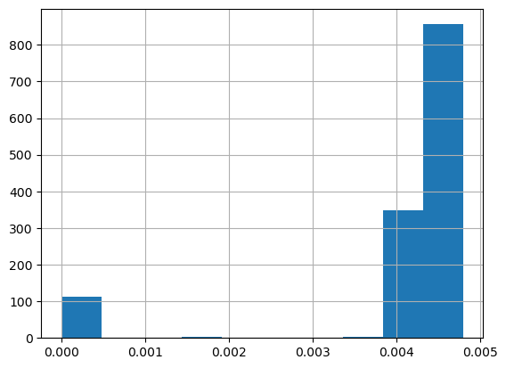
An important caveat here is that in both cases, the idxmin() and idxmax() functions return a single position index number, when in fact the minimum and maximum values may occur multiple times. We can use the value_counts() function to demonstrate that 0 occurs several times in the dataset. Since the dataset is large, we will first subset the data to only include meter readings with very small intervals. Then we will get the count of values across the subset.
low_readings = data[data["INTERVAL_READ"] <= 0.005].copy()
print(pd.value_counts(low_readings["INTERVAL_READ"]))
0.00480    856
0.00420    349
0.00000     72
0.00001     40
0.00360      3
0.00354      1
0.00177      1
0.00240      1
0.00180      1
0.00294      1
Name: INTERVAL_READ, dtype: int64
It’s also helpful to visualize the distribution of values. Pandas has a hist() function for this.
low_readings["INTERVAL_READ"].hist()
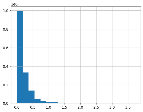
We can plot the distribution of INTERVAL_READ values across the entire dataset. Note that the default behavior in this case is to group the values into 10 bins. The number of bins can be specified using the bins argument.
data["INTERVAL_READ"].hist(bins-20)
To find the number of rows with “INTERVAL_READ” values equal to the minimum or maximum value of that column, we can also create a subset of rows with that value and then get the length of the subset.
print("Number of rows with minimum interval read values:", len(data[data["INTERVAL_READ"] == data["INTERVAL_READ"].min()]))
print("Number of rows with maximum interval read values:", len(data[data["INTERVAL_READ"] == data["INTERVAL_READ"].max()]))
Number of rows with minimum interval read values: 72
Number of rows with maximum interval read values: 1
Grouping data to calculate statistics per smart meter
Up to this point we have been calculating statistics across the entire dataset. This may be useful in some limited circumstances, recall that the dataset consists of data from 15 smart metters over the course of three years. In many cases it will be more useful to calculate statistics per meter. One way to do that would have been to read and analyze the data for each meter individually by reading one file at a time. However, data such as these may often be streamed from multiple meters or other instruments into a single source or database. In these or similar cases it can be more efficient to group data according to specific characteristics.
Our dataset includes a METER_FID field that specifies the identifier of the smart meter from which the data were captured. We can use Pandas’ groupby() method to group data on this field. First we can inspect the number of meters represented in the dataset using the unique() function.
print(data["METER_FID"].unique())
[285 10063 44440 4348 45013 32366 24197 18918 35034 42755 25188 29752 20967 12289 8078]
The output is an array of the unique values in the METER_FID column. We can group the data by these values to essentially create 15 logical subsets of data, with one subset per meter.
meter_data_groups = data.groupby("METER_FID")
print(meter_data_groups.groups.keys())
dict_keys([285, 4348, 8078, 10063, 12289, 18918, 20967, 24197, 25188, 29752, 32366, 35034, 42755, 44440, 45013])
We can use the key or the name of the group to reference a specific group using the get_group() method. Because a group in Pandas is a dataframe, we can operate against groups using the same methods available to any Pandas dataframe.
print(type(meter_data_groups.get_group(285)))
<class 'pandas.core.frame.DataFrame'>
Above, we used the max() function to identify the maximum INTERVAL_READ value within the entire dataset. Using get_group(), we can select the maximum value and other statitics using similar syntax.
print("Maximum value for meter ID 285:", meter_data_groups.get_group(285)["INTERVAL_READ"].max())
print("Sum of values for meter ID 285:", meter_data_groups.get_group(285)["INTERVAL_READ"].sum())
Maximum value for meter ID 285: 2.0526
Sum of values for meter ID 285: 13407.0322
Importantly, we can calculate statistics across all groups at once.
meter_data_groups['INTERVAL_READ'].sum()
METER_FID
285      13407.0322
4348      9854.7946
8078     16979.6884
10063    22628.9866
12289    21175.5478
18918    13790.9044
20967    20488.7761
24197    16401.9134
25188    28962.4688
29752    67684.5526
32366    25832.2660
35034    22653.0976
42755    21882.2350
44440    46950.2104
45013    17184.9206
Name: INTERVAL_READ, dtype: float64
Finally, to calculate multiple statistics we pass a list of the statistics we’re interested in as an argument to the agg() method.
print(meter_data_groups['INTERVAL_READ'].agg([np.sum, np.amax, np.amin, np.mean, np.std]))
                  sum    amax  amin      mean       std
METER_FID
285        13407.0322  2.0526   0.0  0.127671  0.188185
4348        9854.7946  1.4202   0.0  0.093844  0.093136
8078       16979.6884  1.4202   0.0  0.161693  0.158175
10063      22628.9866  2.2284   0.0  0.215490  0.234565
12289      21175.5478  1.4928   0.0  0.201649  0.125956
18918      13790.9044  1.8240   0.0  0.131327  0.153955
20967      20488.7761  1.2522   0.0  0.195109  0.127863
24197      16401.9134  1.4574   0.0  0.156191  0.117501
25188      28962.4688  2.2116   0.0  0.275802  0.259377
29752      67684.5526  3.7092   0.0  0.644541  0.779913
32366      25832.2660  1.5744   0.0  0.245993  0.213024
35034      22653.0976  2.2038   0.0  0.215719  0.157792
42755      21882.2350  2.1780   0.0  0.208378  0.151845
44440      46950.2104  2.2098   0.0  0.447094  0.334872
45013      17184.9206  1.6278   0.0  0.163647  0.148538
Key Points
Use the PANDAS
describe()method to generate descriptive statistics for a dataframe.
Creating a Datetime Index with Pandas
Overview
Teaching: 40 min
Exercises: 20 minQuestions
How can we visualize trends in time series?
Objectives
Use pandas
datetimeindexing to subset time series data.Resample and plot time series statistics.
Calculate and plot rolling averages.
So far we have been interacting with the time series data in ways that are not very different from other tabular datasets. However, time series data can contain unique features that make it difficult to analyze aggregate statistics. For example, the sum of power consumption as measured by a single smart meter over the course of three years may be useful in a limited context, but if we want to analyze the data in order to make predictions about likely demand within one or more households at a given time, we need to account for time features including.
- trends
- seasonality
In this episode, we will use Pandas’ datetime indexing features to illustrate these features.
Setting a datetime index
To begin with we will demonstrate datetime indexing with data from a single meter. First, let’s import the necessary libraries.
import pandas as pd
import matplotlib.pyplot as plt
import glob
import numpy as np
Create the file list as before, but this time read only the first file.
file_list = glob.glob("../data/*.csv")
data = pd.read_csv(file_list[0])
print(data.info())
<class 'pandas.core.frame.DataFrame'>
RangeIndex: 105012 entries, 0 to 105011
Data columns (total 5 columns):
 #   Column         Non-Null Count   Dtype
---  ------         --------------   -----
 0   INTERVAL_TIME  105012 non-null  object
 1   METER_FID      105012 non-null  int64
 2   START_READ     105012 non-null  float64
 3   END_READ       105012 non-null  float64
 4   INTERVAL_READ  105012 non-null  float64
dtypes: float64(3), int64(1), object(1)
memory usage: 4.0+ MB
None
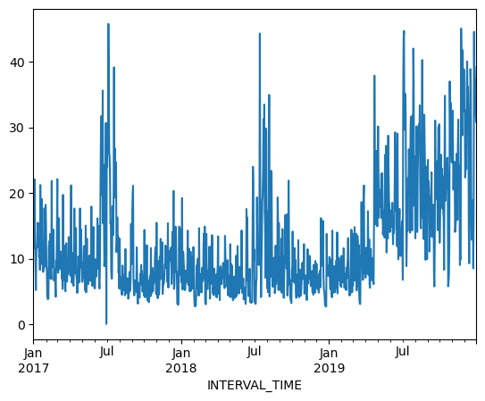
We can plot the INTERVAL_READ values without making any changes to the data. In the image below, we observe what may be trends or seasonality. But we are able to infer this based on our understanding of the data - note that the labels of the X index in the image are the row index positions, not date information.
data["INTERVAL_READ"].plot()
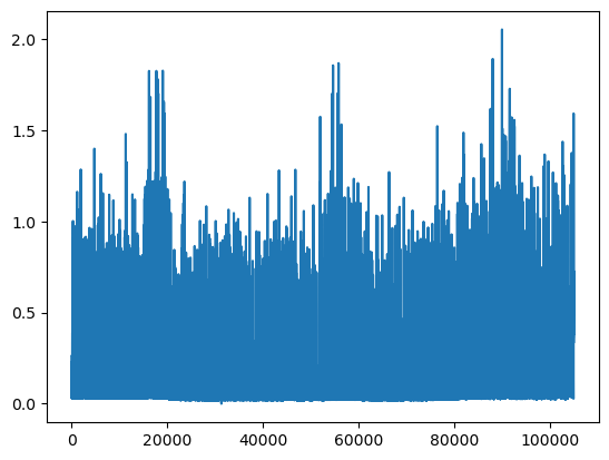
The plot is difficult to read because it is dense. Recall that meter readings are taken every 15 minutes, for a total in the case of this meter of 105,012 readings across the three years of data included in the dataset. In the plot above, we have asked Pandas to plot the value of each one of those readings - that’s a lot of points!
In order to reduce the amount of information and inspect the data for trends and seasonality, the first thing we need to do is set the index of the dataframe to use the INTERVAL_TIME column as a datetime index.
data.set_index(pd.to_datetime(data['INTERVAL_TIME']), inplace=True)
print(data.info())
<class 'pandas.core.frame.DataFrame'>
DatetimeIndex: 105012 entries, 2017-01-01 00:00:00 to 2019-12-31 23:45:00
Data columns (total 5 columns):
 #   Column         Non-Null Count   Dtype
---  ------         --------------   -----
 0   INTERVAL_TIME  105012 non-null  object
 1   METER_FID      105012 non-null  int64
 2   START_READ     105012 non-null  float64
 3   END_READ       105012 non-null  float64
 4   INTERVAL_READ  105012 non-null  float64
dtypes: float64(3), int64(1), object(1)
memory usage: 4.8+ MB
None
Note that the output of the info() function indicates the index is now a DatetimeIndex. However, the INTERVAL_TIME column is still listed as a column, with a data type of object or string.
print(data.head())
                           INTERVAL_TIME  METER_FID  START_READ   END_READ  \
INTERVAL_TIME
2017-01-01 00:00:00  2017-01-01 00:00:00        285   14951.787  14968.082
2017-01-01 00:15:00  2017-01-01 00:15:00        285   14968.082  14979.831
2017-01-01 00:30:00  2017-01-01 00:30:00        285   14968.082  14979.831
2017-01-01 00:45:00  2017-01-01 00:45:00        285   14968.082  14979.831
2017-01-01 01:00:00  2017-01-01 01:00:00        285   14968.082  14979.831

                     INTERVAL_READ
INTERVAL_TIME
2017-01-01 00:00:00         0.0744
2017-01-01 00:15:00         0.0762
2017-01-01 00:30:00         0.1050
2017-01-01 00:45:00         0.0636
2017-01-01 01:00:00         0.0870
Slicing data by date
Now that we have a datetime index for our dataframe, we can use date and time components as labels for label based indexing and slicing. We can use all or part of the datetime information, dependng on how we want to subset the data.
To select data for a single day, we can slice using the date.
one_day_data = data.loc["2017-08-01"].copy()
print(one_day_data.info())
<class 'pandas.core.frame.DataFrame'>
DatetimeIndex: 96 entries, 2017-08-01 00:00:00 to 2017-08-01 23:45:00
Data columns (total 5 columns):
 #   Column         Non-Null Count  Dtype
---  ------         --------------  -----
 0   INTERVAL_TIME  96 non-null     object
 1   METER_FID      96 non-null     int64
 2   START_READ     96 non-null     float64
 3   END_READ       96 non-null     float64
 4   INTERVAL_READ  96 non-null     float64
dtypes: float64(3), int64(1), object(1)
memory usage: 4.5+ KB
None
The info() output above shows that the subset includes 96 readings for a single day, and that the readings were taken between 12AM and 23:45PM. This is expected, based on the structure of the data.
The head() command outputs the first five rows of data.
print(one_day_data.head())
                           INTERVAL_TIME  METER_FID  START_READ   END_READ  \
INTERVAL_TIME
2017-08-01 00:00:00  2017-08-01 00:00:00        285   17563.273  17572.024
2017-08-01 00:15:00  2017-08-01 00:15:00        285   17572.024  17577.448
2017-08-01 00:30:00  2017-08-01 00:30:00        285   17572.024  17577.448
2017-08-01 00:45:00  2017-08-01 00:45:00        285   17572.024  17577.448
2017-08-01 01:00:00  2017-08-01 01:00:00        285   17572.024  17577.448

                     INTERVAL_READ
INTERVAL_TIME
2017-08-01 00:00:00         0.0264
2017-08-01 00:15:00         0.0432
2017-08-01 00:30:00         0.0432
2017-08-01 00:45:00         0.0264
2017-08-01 01:00:00         0.0582
We can inlcude timestamps in the label to subset the data to specific portions of a day. For example, we can inspect power consumption between 8AM and 17:00PM. In this case we use the syntax from before to specify a range for the slice.
print(data.loc["2017-08-01 00:00:00": "2017-08-01 17:00:00"])
                           INTERVAL_TIME  METER_FID  START_READ   END_READ  \
INTERVAL_TIME
2017-08-01 00:00:00  2017-08-01 00:00:00        285   17563.273  17572.024
2017-08-01 00:15:00  2017-08-01 00:15:00        285   17572.024  17577.448
2017-08-01 00:30:00  2017-08-01 00:30:00        285   17572.024  17577.448
2017-08-01 00:45:00  2017-08-01 00:45:00        285   17572.024  17577.448
2017-08-01 01:00:00  2017-08-01 01:00:00        285   17572.024  17577.448
...                                  ...        ...         ...        ...
2017-08-01 16:00:00  2017-08-01 16:00:00        285   17572.024  17577.448
2017-08-01 16:15:00  2017-08-01 16:15:00        285   17572.024  17577.448
2017-08-01 16:30:00  2017-08-01 16:30:00        285   17572.024  17577.448
2017-08-01 16:45:00  2017-08-01 16:45:00        285   17572.024  17577.448
2017-08-01 17:00:00  2017-08-01 17:00:00        285   17572.024  17577.448

                     INTERVAL_READ
INTERVAL_TIME
2017-08-01 00:00:00         0.0264
2017-08-01 00:15:00         0.0432
2017-08-01 00:30:00         0.0432
2017-08-01 00:45:00         0.0264
2017-08-01 01:00:00         0.0582
...                            ...
2017-08-01 16:00:00         0.0540
2017-08-01 16:15:00         0.0288
2017-08-01 16:30:00         0.0462
2017-08-01 16:45:00         0.0360
2017-08-01 17:00:00         0.0378

[69 rows x 5 columns]
We can also slice by month or year. To subset all of the data from 2018 only requires us to include the year in the index label.
print(data.loc["2018"].info())
<class 'pandas.core.frame.DataFrame'>
DatetimeIndex: 35036 entries, 2018-01-01 00:00:00 to 2018-12-31 23:45:00
Data columns (total 5 columns):
 #   Column         Non-Null Count  Dtype
---  ------         --------------  -----
 0   INTERVAL_TIME  35036 non-null  object
 1   METER_FID      35036 non-null  int64
 2   START_READ     35036 non-null  float64
 3   END_READ       35036 non-null  float64
 4   INTERVAL_READ  35036 non-null  float64
dtypes: float64(3), int64(1), object(1)
memory usage: 1.6+ MB
None
The following would subset the data to include days that occurred during the northern hemisphere’s winter of 2018-2019.
print(data.loc["2018-12-21": "2019-03-21"].info())
<class 'pandas.core.frame.DataFrame'>
DatetimeIndex: 8732 entries, 2018-12-21 00:00:00 to 2019-03-21 23:45:00
Data columns (total 5 columns):
 #   Column         Non-Null Count  Dtype
---  ------         --------------  -----
 0   INTERVAL_TIME  8732 non-null   object
 1   METER_FID      8732 non-null   int64
 2   START_READ     8732 non-null   float64
 3   END_READ       8732 non-null   float64
 4   INTERVAL_READ  8732 non-null   float64
dtypes: float64(3), int64(1), object(1)
memory usage: 409.3+ KB
None
Resampling time series
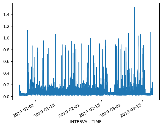
Referring to the above slice of data from December 21, 2018 through March 21, 2019, we can also plot the meter reading values. The result is still noisy, as the plot includes 8732 values taken at 15 minute intervals during that time period. That is still a lot of data to put into a single plot.
print(data.loc["2018-12-21": "2019-03-21"]["INTERVAL_READ"].plot())
Alternatively, we can resample the data to convert readings to a different frequency. That is, instead of a reading every 15 minutes, we can resample to aggregate or group meter readings by hour, day, month, etc. The resample() method has one required argument, which specifies the frequency at which the data should be resampled. For example, to group the data by day, we use an uppercase “D” for this argument
daily_data = data.resample("D")
print(type(daily_data))
<class 'pandas.core.resample.DatetimeIndexResampler'>
Note that the data type of the resampled data is a DatetimeIndexResampler. This is similar to a groupby object in Pandas, and can be accessed using many of the same functions and methods. Previously, we used the max() and min() functions to retrieve maximum and minimum meter readings from the entire dataset. Having resampled the data, we can now retrieve these values per day. Be sure to specify the column against which we want to perform these operations.
print(daily_data['INTERVAL_READ'].min())
INTERVAL_TIME
2017-01-01    0.0282
2017-01-02    0.0366
2017-01-03    0.0300
2017-01-04    0.0288
2017-01-05    0.0288
               ...
2019-12-27    0.0324
2019-12-28    0.0444
2019-12-29    0.0546
2019-12-30    0.0366
2019-12-31    0.0276
Freq: D, Name: INTERVAL_READ, Length: 1095, dtype: float64
We can also plot the results of operations, for example the daily total power consumption.
daily_data["INTERVAL_READ"].sum().plot()
Calculating and plotting rolling averages
Resampling allows us to reduce some of the noise in our plots by aggregating data to a different time frequency. In this way, trends in the data become more evident within our plots. One way we can further amplify trends in time series is through calculating and plotting rolling averages. When we resample data, any statistics are aggregated to the period represented by the resampling frequency. In our example above, the data were resampled per day. As a result our minimum and maximum values, or any other statistics, are calculated per day. By contrast, rolling means allow us to calcuate averages across days.
To demonstrate, we will resample our December 21, 2018 - March 21, 2019 subset and compare daily total power consumption with a rolling average of power consumption per week.
winter_18 = data.loc["2018-12-21": "2019-03-21"].copy()
print(winter_18.info())
<class 'pandas.core.frame.DataFrame'>
DatetimeIndex: 8732 entries, 2018-12-21 00:00:00 to 2019-03-21 23:45:00
Data columns (total 5 columns):
 #   Column         Non-Null Count  Dtype
---  ------         --------------  -----
 0   INTERVAL_TIME  8732 non-null   object
 1   METER_FID      8732 non-null   int64
 2   START_READ     8732 non-null   float64
 3   END_READ       8732 non-null   float64
 4   INTERVAL_READ  8732 non-null   float64
dtypes: float64(3), int64(1), object(1)
memory usage: 409.3+ KB
None
With the resampled data, we can calculate daily total power consumption using the sum()function. The head() command is used below to view the first 14 rows of output.
print(winter_18_daily["INTERVAL_READ"].sum().head(14))
INTERVAL_TIME
2018-12-21     4.2462
2018-12-22     2.8758
2018-12-23     2.7906
2018-12-24     2.7930
2018-12-25     2.6748
2018-12-26    13.7778
2018-12-27     9.3912
2018-12-28     7.4262
2018-12-29     7.9764
2018-12-30     8.9406
2018-12-31     7.3674
2019-01-01     7.5324
2019-01-02    10.2534
2019-01-03     6.8544
Freq: D, Name: INTERVAL_READ, dtype: float64
To calculate a rolling seven day statistic, we use the Numpy rolling() function. The window argument specifies how many timesteps we are calculating the rolling statistic across. Since our data have been resampled at a per day frequency, a single timestep is one day. Passing a value of 7 to the window argument means that we will be calculating a statistic across every seven days, or weekly. In order to calculate averages, the result of the rolling() function is then passed to the mean() function. For the sake of comparison we will also huse the head() function to output the first 14 rows of the result.
print(winter_18_daily["INTERVAL_READ"].sum().rolling(window=7).mean().head(14))
INTERVAL_TIME
2018-12-21         NaN
2018-12-22         NaN
2018-12-23         NaN
2018-12-24         NaN
2018-12-25         NaN
2018-12-26         NaN
2018-12-27    5.507057
2018-12-28    5.961343
2018-12-29    6.690000
2018-12-30    7.568571
2018-12-31    8.222057
2019-01-01    8.916000
2019-01-02    8.412514
2019-01-03    8.050114
Freq: D, Name: INTERVAL_READ, dtype: float64
Note that the first six rows of output are not a number, or NaN. This is because setting a window of 7 for our rolling average meant that there were not enough days from which to calculate an average between December 21 and 26. Beginning with December 27, a seven day average can be calculated using the daily total power consumption between December 21 and 27. On December 28, the average is calculated using the daily total power consumption between December 22 and 28, etc. We can verify this by manually calculating the 7 day average between December 21 and 27 and comparing it with the value given above:
print((4.2462 + 2.8758 + 2.7906 + 2.7930 + 2.6748 + 13.7778 + 9.3912) / 7)
5.507057142857143
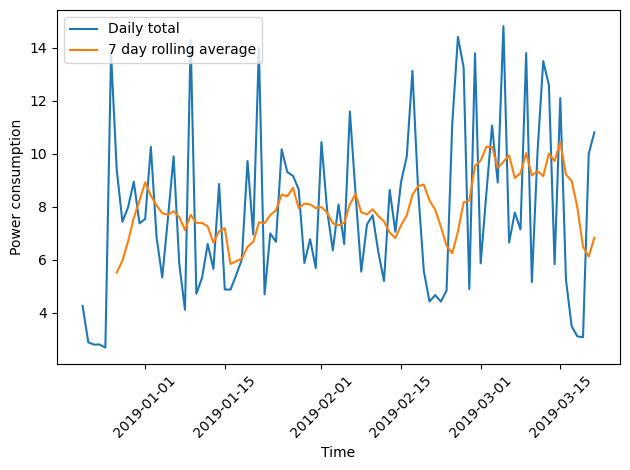
Plotting the daily total and the weekly average together demonstrates how the rolling average smooths the data and can make trends more apparent.
fig, ax = plt.subplots()

ax.plot(winter_18_daily["INTERVAL_READ"].sum(), label="Daily total")
ax.plot(winter_18_daily["INTERVAL_READ"].sum().rolling(window=7).mean(), label="7 day rolling average")

ax.legend(loc=2)

ax.set_xlabel("Time")
ax.set_ylabel("Power consumption")

plt.xticks(rotation=45)
plt.tight_layout()
Key Points
Use
resample()on a datetime index to calculate aggregate statistics across time series.