Creating a Datetime Index with Pandas
Overview
Teaching: 40 min
Exercises: 20 minQuestions
How can we visualize trends in time series?
Objectives
Use pandas
datetimeindexing to subset time series data.Resample and plot time series statistics.
Calculate and plot rolling averages.
So far we have been interacting with the time series data in ways that are not very different from other tabular datasets. However, time series data can contain unique features that make it difficult to analyze aggregate statistics. For example, the sum of power consumption as measured by a single smart meter over the course of three years may be useful in a limited context, but if we want to analyze the data in order to make predictions about likely demand within one or more households at a given time, we need to account for time features including.
- trends
- seasonality
In this episode, we will use Pandas’ datetime indexing features to illustrate these features.
Setting a datetime index
To begin with we will demonstrate datetime indexing with data from a single meter. First, let’s import the necessary libraries.
import pandas as pd
import matplotlib.pyplot as plt
import glob
import numpy as np
Create the file list as before, but this time read only the first file.
file_list = glob.glob("../data/*.csv")
data = pd.read_csv(file_list[0])
print(data.info())
<class 'pandas.core.frame.DataFrame'>
RangeIndex: 105012 entries, 0 to 105011
Data columns (total 5 columns):
 #   Column         Non-Null Count   Dtype
---  ------         --------------   -----
 0   INTERVAL_TIME  105012 non-null  object
 1   METER_FID      105012 non-null  int64
 2   START_READ     105012 non-null  float64
 3   END_READ       105012 non-null  float64
 4   INTERVAL_READ  105012 non-null  float64
dtypes: float64(3), int64(1), object(1)
memory usage: 4.0+ MB
None
We can plot the INTERVAL_READ values without making any changes to the data. In the image below, we observe what may be trends or seasonality. But we are able to infer this based on our understanding of the data - note that the labels of the X index in the image are the row index positions, not date information.
data["INTERVAL_READ"].plot()
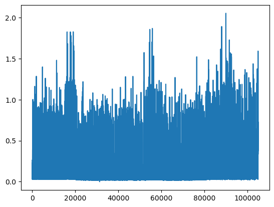
The plot is difficult to read because it is dense. Recall that meter readings are taken every 15 minutes, for a total in the case of this meter of 105,012 readings across the three years of data included in the dataset. In the plot above, we have asked Pandas to plot the value of each one of those readings - that’s a lot of points!
In order to reduce the amount of information and inspect the data for trends and seasonality, the first thing we need to do is set the index of the dataframe to use the INTERVAL_TIME column as a datetime index.
data.set_index(pd.to_datetime(data['INTERVAL_TIME']), inplace=True)
print(data.info())
<class 'pandas.core.frame.DataFrame'>
DatetimeIndex: 105012 entries, 2017-01-01 00:00:00 to 2019-12-31 23:45:00
Data columns (total 5 columns):
 #   Column         Non-Null Count   Dtype
---  ------         --------------   -----
 0   INTERVAL_TIME  105012 non-null  object
 1   METER_FID      105012 non-null  int64
 2   START_READ     105012 non-null  float64
 3   END_READ       105012 non-null  float64
 4   INTERVAL_READ  105012 non-null  float64
dtypes: float64(3), int64(1), object(1)
memory usage: 4.8+ MB
None
Note that the output of the info() function indicates the index is now a DatetimeIndex. However, the INTERVAL_TIME column is still listed as a column, with a data type of object or string.
print(data.head())
                           INTERVAL_TIME  METER_FID  START_READ   END_READ  \
INTERVAL_TIME
2017-01-01 00:00:00  2017-01-01 00:00:00        285   14951.787  14968.082
2017-01-01 00:15:00  2017-01-01 00:15:00        285   14968.082  14979.831
2017-01-01 00:30:00  2017-01-01 00:30:00        285   14968.082  14979.831
2017-01-01 00:45:00  2017-01-01 00:45:00        285   14968.082  14979.831
2017-01-01 01:00:00  2017-01-01 01:00:00        285   14968.082  14979.831

                     INTERVAL_READ
INTERVAL_TIME
2017-01-01 00:00:00         0.0744
2017-01-01 00:15:00         0.0762
2017-01-01 00:30:00         0.1050
2017-01-01 00:45:00         0.0636
2017-01-01 01:00:00         0.0870
Slicing data by date
Now that we have a datetime index for our dataframe, we can use date and time components as labels for label based indexing and slicing. We can use all or part of the datetime information, dependng on how we want to subset the data.
To select data for a single day, we can slice using the date.
one_day_data = data.loc["2017-08-01"].copy()
print(one_day_data.info())
<class 'pandas.core.frame.DataFrame'>
DatetimeIndex: 96 entries, 2017-08-01 00:00:00 to 2017-08-01 23:45:00
Data columns (total 5 columns):
 #   Column         Non-Null Count  Dtype
---  ------         --------------  -----
 0   INTERVAL_TIME  96 non-null     object
 1   METER_FID      96 non-null     int64
 2   START_READ     96 non-null     float64
 3   END_READ       96 non-null     float64
 4   INTERVAL_READ  96 non-null     float64
dtypes: float64(3), int64(1), object(1)
memory usage: 4.5+ KB
None
The info() output above shows that the subset includes 96 readings for a single day, and that the readings were taken between 12AM and 23:45PM. This is expected, based on the structure of the data.
The head() command outputs the first five rows of data.
print(one_day_data.head())
                           INTERVAL_TIME  METER_FID  START_READ   END_READ  \
INTERVAL_TIME
2017-08-01 00:00:00  2017-08-01 00:00:00        285   17563.273  17572.024
2017-08-01 00:15:00  2017-08-01 00:15:00        285   17572.024  17577.448
2017-08-01 00:30:00  2017-08-01 00:30:00        285   17572.024  17577.448
2017-08-01 00:45:00  2017-08-01 00:45:00        285   17572.024  17577.448
2017-08-01 01:00:00  2017-08-01 01:00:00        285   17572.024  17577.448

                     INTERVAL_READ
INTERVAL_TIME
2017-08-01 00:00:00         0.0264
2017-08-01 00:15:00         0.0432
2017-08-01 00:30:00         0.0432
2017-08-01 00:45:00         0.0264
2017-08-01 01:00:00         0.0582
We can inlcude timestamps in the label to subset the data to specific portions of a day. For example, we can inspect power consumption between 8AM and 17:00PM. In this case we use the syntax from before to specify a range for the slice.
print(data.loc["2017-08-01 00:00:00": "2017-08-01 17:00:00"])
                           INTERVAL_TIME  METER_FID  START_READ   END_READ  \
INTERVAL_TIME
2017-08-01 00:00:00  2017-08-01 00:00:00        285   17563.273  17572.024
2017-08-01 00:15:00  2017-08-01 00:15:00        285   17572.024  17577.448
2017-08-01 00:30:00  2017-08-01 00:30:00        285   17572.024  17577.448
2017-08-01 00:45:00  2017-08-01 00:45:00        285   17572.024  17577.448
2017-08-01 01:00:00  2017-08-01 01:00:00        285   17572.024  17577.448
...                                  ...        ...         ...        ...
2017-08-01 16:00:00  2017-08-01 16:00:00        285   17572.024  17577.448
2017-08-01 16:15:00  2017-08-01 16:15:00        285   17572.024  17577.448
2017-08-01 16:30:00  2017-08-01 16:30:00        285   17572.024  17577.448
2017-08-01 16:45:00  2017-08-01 16:45:00        285   17572.024  17577.448
2017-08-01 17:00:00  2017-08-01 17:00:00        285   17572.024  17577.448

                     INTERVAL_READ
INTERVAL_TIME
2017-08-01 00:00:00         0.0264
2017-08-01 00:15:00         0.0432
2017-08-01 00:30:00         0.0432
2017-08-01 00:45:00         0.0264
2017-08-01 01:00:00         0.0582
...                            ...
2017-08-01 16:00:00         0.0540
2017-08-01 16:15:00         0.0288
2017-08-01 16:30:00         0.0462
2017-08-01 16:45:00         0.0360
2017-08-01 17:00:00         0.0378

[69 rows x 5 columns]
We can also slice by month or year. To subset all of the data from 2018 only requires us to include the year in the index label.
print(data.loc["2018"].info())
<class 'pandas.core.frame.DataFrame'>
DatetimeIndex: 35036 entries, 2018-01-01 00:00:00 to 2018-12-31 23:45:00
Data columns (total 5 columns):
 #   Column         Non-Null Count  Dtype
---  ------         --------------  -----
 0   INTERVAL_TIME  35036 non-null  object
 1   METER_FID      35036 non-null  int64
 2   START_READ     35036 non-null  float64
 3   END_READ       35036 non-null  float64
 4   INTERVAL_READ  35036 non-null  float64
dtypes: float64(3), int64(1), object(1)
memory usage: 1.6+ MB
None
The following would subset the data to include days that occurred during the northern hemisphere’s winter of 2018-2019.
print(data.loc["2018-12-21": "2019-03-21"].info())
<class 'pandas.core.frame.DataFrame'>
DatetimeIndex: 8732 entries, 2018-12-21 00:00:00 to 2019-03-21 23:45:00
Data columns (total 5 columns):
 #   Column         Non-Null Count  Dtype
---  ------         --------------  -----
 0   INTERVAL_TIME  8732 non-null   object
 1   METER_FID      8732 non-null   int64
 2   START_READ     8732 non-null   float64
 3   END_READ       8732 non-null   float64
 4   INTERVAL_READ  8732 non-null   float64
dtypes: float64(3), int64(1), object(1)
memory usage: 409.3+ KB
None
Resampling time series
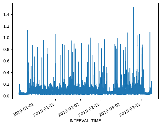
Referring to the above slice of data from December 21, 2018 through March 21, 2019, we can also plot the meter reading values. The result is still noisy, as the plot includes 8732 values taken at 15 minute intervals during that time period. That is still a lot of data to put into a single plot.
print(data.loc["2018-12-21": "2019-03-21"]["INTERVAL_READ"].plot())
Alternatively, we can resample the data to convert readings to a different frequency. That is, instead of a reading every 15 minutes, we can resample to aggregate or group meter readings by hour, day, month, etc. The resample() method has one required argument, which specifies the frequency at which the data should be resampled. For example, to group the data by day, we use an uppercase “D” for this argument
daily_data = data.resample("D")
print(type(daily_data))
<class 'pandas.core.resample.DatetimeIndexResampler'>
Note that the data type of the resampled data is a DatetimeIndexResampler. This is similar to a groupby object in Pandas, and can be accessed using many of the same functions and methods. Previously, we used the max() and min() functions to retrieve maximum and minimum meter readings from the entire dataset. Having resampled the data, we can now retrieve these values per day. Be sure to specify the column against which we want to perform these operations.
print(daily_data['INTERVAL_READ'].min())
INTERVAL_TIME
2017-01-01    0.0282
2017-01-02    0.0366
2017-01-03    0.0300
2017-01-04    0.0288
2017-01-05    0.0288
               ...
2019-12-27    0.0324
2019-12-28    0.0444
2019-12-29    0.0546
2019-12-30    0.0366
2019-12-31    0.0276
Freq: D, Name: INTERVAL_READ, Length: 1095, dtype: float64
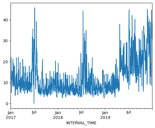
We can also plot the results of operations, for example the daily total power consumption.
daily_data["INTERVAL_READ"].sum().plot()
Calculating and plotting rolling averages
Resampling allows us to reduce some of the noise in our plots by aggregating data to a different time frequency. In this way, trends in the data become more evident within our plots. One way we can further amplify trends in time series is through calculating and plotting rolling averages. When we resample data, any statistics are aggregated to the period represented by the resampling frequency. In our example above, the data were resampled per day. As a result our minimum and maximum values, or any other statistics, are calculated per day. By contrast, rolling means allow us to calcuate averages across days.
To demonstrate, we will resample our December 21, 2018 - March 21, 2019 subset and compare daily total power consumption with a rolling average of power consumption per week.
winter_18 = data.loc["2018-12-21": "2019-03-21"].copy()
print(winter_18.info())
<class 'pandas.core.frame.DataFrame'>
DatetimeIndex: 8732 entries, 2018-12-21 00:00:00 to 2019-03-21 23:45:00
Data columns (total 5 columns):
 #   Column         Non-Null Count  Dtype
---  ------         --------------  -----
 0   INTERVAL_TIME  8732 non-null   object
 1   METER_FID      8732 non-null   int64
 2   START_READ     8732 non-null   float64
 3   END_READ       8732 non-null   float64
 4   INTERVAL_READ  8732 non-null   float64
dtypes: float64(3), int64(1), object(1)
memory usage: 409.3+ KB
None
With the resampled data, we can calculate daily total power consumption using the sum()function. The head() command is used below to view the first 14 rows of output.
print(winter_18_daily["INTERVAL_READ"].sum().head(14))
INTERVAL_TIME
2018-12-21     4.2462
2018-12-22     2.8758
2018-12-23     2.7906
2018-12-24     2.7930
2018-12-25     2.6748
2018-12-26    13.7778
2018-12-27     9.3912
2018-12-28     7.4262
2018-12-29     7.9764
2018-12-30     8.9406
2018-12-31     7.3674
2019-01-01     7.5324
2019-01-02    10.2534
2019-01-03     6.8544
Freq: D, Name: INTERVAL_READ, dtype: float64
To calculate a rolling seven day statistic, we use the Numpy rolling() function. The window argument specifies how many timesteps we are calculating the rolling statistic across. Since our data have been resampled at a per day frequency, a single timestep is one day. Passing a value of 7 to the window argument means that we will be calculating a statistic across every seven days, or weekly. In order to calculate averages, the result of the rolling() function is then passed to the mean() function. For the sake of comparison we will also huse the head() function to output the first 14 rows of the result.
print(winter_18_daily["INTERVAL_READ"].sum().rolling(window=7).mean().head(14))
INTERVAL_TIME
2018-12-21         NaN
2018-12-22         NaN
2018-12-23         NaN
2018-12-24         NaN
2018-12-25         NaN
2018-12-26         NaN
2018-12-27    5.507057
2018-12-28    5.961343
2018-12-29    6.690000
2018-12-30    7.568571
2018-12-31    8.222057
2019-01-01    8.916000
2019-01-02    8.412514
2019-01-03    8.050114
Freq: D, Name: INTERVAL_READ, dtype: float64
Note that the first six rows of output are not a number, or NaN. This is because setting a window of 7 for our rolling average meant that there were not enough days from which to calculate an average between December 21 and 26. Beginning with December 27, a seven day average can be calculated using the daily total power consumption between December 21 and 27. On December 28, the average is calculated using the daily total power consumption between December 22 and 28, etc. We can verify this by manually calculating the 7 day average between December 21 and 27 and comparing it with the value given above:
print((4.2462 + 2.8758 + 2.7906 + 2.7930 + 2.6748 + 13.7778 + 9.3912) / 7)
5.507057142857143
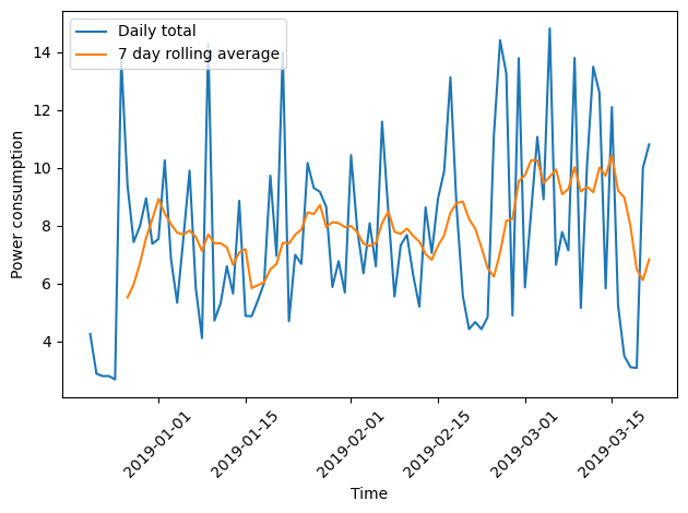
Plotting the daily total and the weekly average together demonstrates how the rolling average smooths the data and can make trends more apparent.
fig, ax = plt.subplots()

ax.plot(winter_18_daily["INTERVAL_READ"].sum(), label="Daily total")
ax.plot(winter_18_daily["INTERVAL_READ"].sum().rolling(window=7).mean(), label="7 day rolling average")

ax.legend(loc=2)

ax.set_xlabel("Time")
ax.set_ylabel("Power consumption")

plt.xticks(rotation=45)
plt.tight_layout()
Key Points
Use
resample()on a datetime index to calculate aggregate statistics across time series.