Summarizing Tabular Data with PANDAS
Overview
Teaching: 30 min
Exercises: 15 minQuestions
How can we summarize large datasets?
Objectives
Summarize large datasets using descriptive statistics.
Perform operations to identify outliers in tabular data.
Metadata provided with the published Los Alamos Public Utility Department Smart Meter dataset at Dryad https://doi.org/10.5061/dryad.m0cfxpp2c indicates that aside from de-identification the data have not been pre-processed or normalized and may include missing data, duplicate entries, and other anomalies.
The full dataset is too large for this tutorial format. The subset used for the lesson has been cleaned to elminate null and duplicate values, but may still contain outliers or erroneous meter readings. One way to identify potential errors within a dataset is to inspect the data using descriptive statistics.
Descriptive Statistics
Descriptive statistics provide us with a means to summarize large datasets, and to identify the presence of outliers, missing data, etc.
First, import Pandas and the glob library, which provides utilities for generating lists of files that match specific file name patterns.
import pandas as pd
import glob
import numpy as np
Next, use the glob function to create a list of files that Pandas will combine into a single data frame.
file_list = glob.glob("../data/*.csv")
file_list
['../data\\ladpu_smart_meter_data_01.csv',
 '../data\\ladpu_smart_meter_data_02.csv',
 '../data\\ladpu_smart_meter_data_03.csv',
 '../data\\ladpu_smart_meter_data_04.csv',
 '../data\\ladpu_smart_meter_data_05.csv',
 '../data\\ladpu_smart_meter_data_06.csv',
 '../data\\ladpu_smart_meter_data_07.csv',
 '../data\\ladpu_smart_meter_data_08.csv',
 '../data\\ladpu_smart_meter_data_09.csv',
 '../data\\ladpu_smart_meter_data_10.csv',
 '../data\\ladpu_smart_meter_data_11.csv',
 '../data\\ladpu_smart_meter_data_12.csv',
 '../data\\ladpu_smart_meter_data_13.csv',
 '../data\\ladpu_smart_meter_data_14.csv',
 '../data\\ladpu_smart_meter_data_15.csv']
As before, concatenate all of the individual CSV files into a single dataframe and reset the index.
data = pd.concat([pd.read_csv(f) for f in file_list])
data.reset_index(inplace=True, drop=True)
print(data.axes)
[RangeIndex(start=0, stop=1575180, step=1), Index(['INTERVAL_TIME', 'METER_FID', 'START_READ', 'END_READ',
       'INTERVAL_READ'],
      dtype='object')]
print(data.info())
<class 'pandas.core.frame.DataFrame'>
RangeIndex: 1575180 entries, 0 to 1575179
Data columns (total 5 columns):
 #   Column         Non-Null Count    Dtype
---  ------         --------------    -----
 0   INTERVAL_TIME  1575180 non-null  object
 1   METER_FID      1575180 non-null  int64
 2   START_READ     1575180 non-null  float64
 3   END_READ       1575180 non-null  float64
 4   INTERVAL_READ  1575180 non-null  float64
dtypes: float64(3), int64(1), object(1)
memory usage: 60.1+ MB
None
In a later episode we will create a datetime index using the INTERVAL_TIME field. For now we will change the data type of INTERVAL_TIME to datetime and store the updated data in an iso_date column.
data["iso_date"] = pd.to_datetime(data["INTERVAL_TIME"], infer_datetime_format=True)
print(data.info())
<class 'pandas.core.frame.DataFrame'>
RangeIndex: 1575180 entries, 0 to 1575179
Data columns (total 6 columns):
 #   Column         Non-Null Count    Dtype
---  ------         --------------    -----
 0   INTERVAL_TIME  1575180 non-null  object
 1   METER_FID      1575180 non-null  int64
 2   START_READ     1575180 non-null  float64
 3   END_READ       1575180 non-null  float64
 4   INTERVAL_READ  1575180 non-null  float64
 5   iso_date       1575180 non-null  datetime64[ns]
dtypes: datetime64[ns](1), float64(3), int64(1), object(1)
memory usage: 72.1+ MB
None
The output of the info() method above indicates that four of the columns in the dataframe have numeric data types: “METER_FID”, “START_READ”, “END_READ”, and “INTERVAL_READ”. By default, Pandas will calculate descriptive statistics for numeric data types within a dataset.
print(data.describe())
          METER_FID    START_READ      END_READ  INTERVAL_READ
count  1.575180e+06  1.575180e+06  1.575180e+06   1.575180e+06
mean   2.357953e+04  3.733560e+04  3.734571e+04   2.322766e-01
std    1.414977e+04  1.877812e+04  1.877528e+04   3.026917e-01
min    2.850000e+02  7.833000e+00  7.833000e+00   0.000000e+00
25%    1.006300e+04  2.583424e+04  2.584509e+04   8.820000e-02
50%    2.419700e+04  3.399917e+04  3.401764e+04   1.452000e-01
75%    3.503400e+04  4.391686e+04  4.393681e+04   2.490000e-01
max    4.501300e+04  9.997330e+04  9.997330e+04   3.709200e+00
Since the values for “START_READ” and “END_READ” are calculated across fifteen different meters over a period of three years, those statistics may not be useful or of interest. Without grouping or otherwise manipulating the data, the only statistics that may be informative in the aggregate are for the “INTERVAL_READ” variable. This is the variable that measures actual power consumption per time intervals of 15 minutes.
Also note that “METER_FID” is treated as an integer by Pandas. This is reasonable, since the identifiers are whole numbers. However, since these identifiers aren’t treated numerically in our analysis we can change the data type to object. We will see below how this affects the way statistics are calculated.
data = data.astype({"METER_FID": "object"})
print(data.dtypes)
INTERVAL_TIME            object
METER_FID                object
START_READ              float64
END_READ                float64
INTERVAL_READ           float64
iso_date         datetime64[ns]
dtype: object
If we re-run the code print(data.describe()) as above, Pandas will now exclude information about “METER_FID”, since by default Pandas only outputs descriptive statistics for numeric data types. We can change the default behavior to include statistics for all columns.
print(data.describe(include="all", datetime_is_numeric=True))
              INTERVAL_TIME  METER_FID    START_READ      END_READ  \
count               1575180  1575180.0  1.575180e+06  1.575180e+06
unique               105012       15.0           NaN           NaN
top     2017-01-01 00:00:00      285.0           NaN           NaN
freq                     15   105012.0           NaN           NaN
mean                    NaN        NaN  3.733560e+04  3.734571e+04
min                     NaN        NaN  7.833000e+00  7.833000e+00
25%                     NaN        NaN  2.583424e+04  2.584509e+04
50%                     NaN        NaN  3.399917e+04  3.401764e+04
75%                     NaN        NaN  4.391686e+04  4.393681e+04
max                     NaN        NaN  9.997330e+04  9.997330e+04
std                     NaN        NaN  1.877812e+04  1.877528e+04

        INTERVAL_READ                       iso_date
count    1.575180e+06                        1575180
unique            NaN                            NaN
top               NaN                            NaN
freq              NaN                            NaN
mean     2.322766e-01  2018-07-02 20:14:16.239287296
min      0.000000e+00            2017-01-01 00:00:00
25%      8.820000e-02            2017-10-02 12:11:15
50%      1.452000e-01            2018-07-03 00:22:30
75%      2.490000e-01            2019-04-02 12:33:45
max      3.709200e+00            2019-12-31 23:45:00
std      3.026917e-01                            NaN
For non-numeric data types, Pandas has included statistics for count, unique, top, and freq. Respectively, these represent the total number of observations, the number of uniquely occuring values, the most commonly occuring value, and the number of time the most commonly occurring value appears in the dataset.
We can view the descriptive statistics for a single column:
print(data["INTERVAL_READ"].describe())
count    1.575180e+06
mean     2.322766e-01
std      3.026917e-01
min      0.000000e+00
25%      8.820000e-02
50%      1.452000e-01
75%      2.490000e-01
max      3.709200e+00
Name: INTERVAL_READ, dtype: float64
We notice the difference between the value given for 75% range and the maximum meter reading is larger than the differences between the other percentiles. For a closer inspection of high readings, we can also specify percentiles.
print(data["INTERVAL_READ"].describe(percentiles = [0.75, 0.85, 0.95, 0.99]))
count    1.575180e+06
mean     2.322766e-01
std      3.026917e-01
min      0.000000e+00
50%      1.452000e-01
75%      2.490000e-01
85%      3.846000e-01
95%      6.912000e-01
99%      1.714926e+00
max      3.709200e+00
Name: INTERVAL_READ, dtype: float64
There seem to be some meter readings that are unusually high between the 95% percentile and the maximum. We will investgate this in more detail below.
Challenge: Descriptive Statistics by Data Type
We have seen that the default behavior in Pandas is to output descriptive statistics for numeric data types. It is also possible, using the
includeargument demonstrated above, to output descriptive statistics for specific data types.Write some code to output descriptive statistics by data type for each of the data types in the dataset. Refer to python data types documentation and use any of the methods we have demonstrated to identify the data types of different columns in a pandas dataframe.
Solution
print("Dataframe info:")
print(data.info())

Dataframe info:
<class 'pandas.core.frame.DataFrame'>
RangeIndex: 1575180 entries, 0 to 1575179
Data columns (total 6 columns):
 #   Column         Non-Null Count    Dtype
---  ------         --------------    -----
 0   INTERVAL_TIME  1575180 non-null  object
 1   METER_FID      1575180 non-null  object
 2   START_READ     1575180 non-null  float64
 3   END_READ       1575180 non-null  float64
 4   INTERVAL_READ  1575180 non-null  float64
 5   iso_date       1575180 non-null  datetime64[ns]
dtypes: datetime64[ns](1), float64(3), object(2)
memory usage: 72.1+ MB
None

print("Descriptive stats for floating point numbers:")
print(data.describe(include=float))

Descriptive stats for floating point numbers:
         START_READ      END_READ  INTERVAL_READ
count  1.575180e+06  1.575180e+06   1.575180e+06
mean   3.733560e+04  3.734571e+04   2.322766e-01
std    1.877812e+04  1.877528e+04   3.026917e-01
min    7.833000e+00  7.833000e+00   0.000000e+00
25%    2.583424e+04  2.584509e+04   8.820000e-02
50%    3.399917e+04  3.401764e+04   1.452000e-01
75%    4.391686e+04  4.393681e+04   2.490000e-01
max    9.997330e+04  9.997330e+04   3.709200e+00

print("Descriptive stats for objects:")
print(data.describe(include=object))

Descriptive stats for objects:
              INTERVAL_TIME  METER_FID
count               1575180    1575180
unique               105012         15
top     2017-01-01 00:00:00        285
freq                     15     105012
Working with Values
Returning to our descriptive statistics, we have already noted that the maximum value is well above the 99th percentile. Our minimum value of zero may also be unusual, since many homes might be expected to use some amount of energy every fifteen minutes, even when residents are away.
print(data["INTERVAL_READ"].describe())
count    1.575180e+06
mean     2.322766e-01
std      3.026917e-01
min      0.000000e+00
25%      8.820000e-02
50%      1.452000e-01
75%      2.490000e-01
max      3.709200e+00
Name: INTERVAL_READ, dtype: float64
We can also select the minimum and maximum values in a column using the min() and max() functions.
print("Minimum value:", data["INTERVAL_READ"].min())
print("Maximum value:", data["INTERVAL_READ"].max())
Minimum value: 0.0
Maximum value: 3.7092
This is useful if we want to know what those values are. We may want to have more information about the corresponding meter’s start and end reading, the date, and the meter ID. One way to discover this information is to use the idxmin() and idxmax() functions to get the position indices of the rows where the minimum and maximum values occur.
print("Position index of the minimum value:", data["INTERVAL_READ"].idxmin())
print("Position index of the maximum value:", data["INTERVAL_READ"].idxmax())
Position index of the minimum value: 31315
Position index of the maximum value: 1187650
Now we can use the position index to select the row with the reported minimum value.
print(data.iloc[31315])
INTERVAL_TIME    2017-11-24 05:45:00
METER_FID                        285
START_READ                 18409.997
END_READ                   18418.554
INTERVAL_READ                    0.0
iso_date         2017-11-24 05:45:00
Name: 31315, dtype: object
We can do the same with the maximum value.
print(data.iloc[1187650])
INTERVAL_TIME    2017-12-06 18:30:00
METER_FID                      29752
START_READ                 99685.954
END_READ                   99788.806
INTERVAL_READ                 3.7092
iso_date         2017-12-06 18:30:00
Name: 1187650, dtype: object
An important caveat here is that in both cases, the idxmin() and idxmax() functions return a single position index number, when in fact the minimum and maximum values may occur multiple times. We can use the value_counts() function to demonstrate that 0 occurs several times in the dataset. Since the dataset is large, we will first subset the data to only include meter readings with very small intervals. Then we will get the count of values across the subset.
low_readings = data[data["INTERVAL_READ"] <= 0.005].copy()
print(pd.value_counts(low_readings["INTERVAL_READ"]))
0.00480    856
0.00420    349
0.00000     72
0.00001     40
0.00360      3
0.00354      1
0.00177      1
0.00240      1
0.00180      1
0.00294      1
Name: INTERVAL_READ, dtype: int64
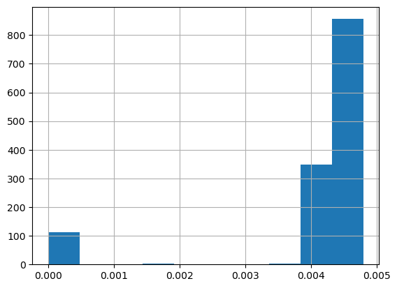
It’s also helpful to visualize the distribution of values. Pandas has a hist() function for this.
low_readings["INTERVAL_READ"].hist()
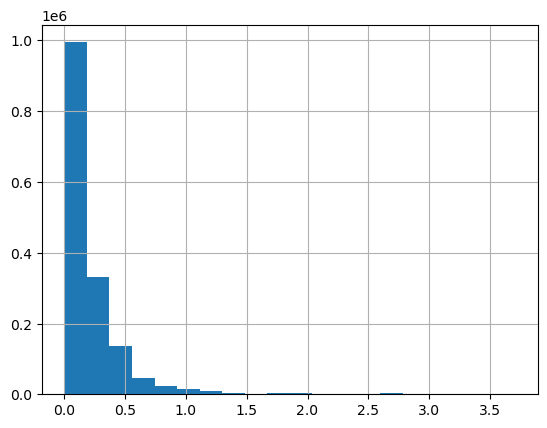
We can plot the distribution of INTERVAL_READ values across the entire dataset. Note that the default behavior in this case is to group the values into 10 bins. The number of bins can be specified using the bins argument.
data["INTERVAL_READ"].hist(bins-20)
To find the number of rows with “INTERVAL_READ” values equal to the minimum or maximum value of that column, we can also create a subset of rows with that value and then get the length of the subset.
print("Number of rows with minimum interval read values:", len(data[data["INTERVAL_READ"] == data["INTERVAL_READ"].min()]))
print("Number of rows with maximum interval read values:", len(data[data["INTERVAL_READ"] == data["INTERVAL_READ"].max()]))
Number of rows with minimum interval read values: 72
Number of rows with maximum interval read values: 1
Grouping data to calculate statistics per smart meter
Up to this point we have been calculating statistics across the entire dataset. This may be useful in some limited circumstances, recall that the dataset consists of data from 15 smart metters over the course of three years. In many cases it will be more useful to calculate statistics per meter. One way to do that would have been to read and analyze the data for each meter individually by reading one file at a time. However, data such as these may often be streamed from multiple meters or other instruments into a single source or database. In these or similar cases it can be more efficient to group data according to specific characteristics.
Our dataset includes a METER_FID field that specifies the identifier of the smart meter from which the data were captured. We can use Pandas’ groupby() method to group data on this field. First we can inspect the number of meters represented in the dataset using the unique() function.
print(data["METER_FID"].unique())
[285 10063 44440 4348 45013 32366 24197 18918 35034 42755 25188 29752 20967 12289 8078]
The output is an array of the unique values in the METER_FID column. We can group the data by these values to essentially create 15 logical subsets of data, with one subset per meter.
meter_data_groups = data.groupby("METER_FID")
print(meter_data_groups.groups.keys())
dict_keys([285, 4348, 8078, 10063, 12289, 18918, 20967, 24197, 25188, 29752, 32366, 35034, 42755, 44440, 45013])
We can use the key or the name of the group to reference a specific group using the get_group() method. Because a group in Pandas is a dataframe, we can operate against groups using the same methods available to any Pandas dataframe.
print(type(meter_data_groups.get_group(285)))
<class 'pandas.core.frame.DataFrame'>
Above, we used the max() function to identify the maximum INTERVAL_READ value within the entire dataset. Using get_group(), we can select the maximum value and other statitics using similar syntax.
print("Maximum value for meter ID 285:", meter_data_groups.get_group(285)["INTERVAL_READ"].max())
print("Sum of values for meter ID 285:", meter_data_groups.get_group(285)["INTERVAL_READ"].sum())
Maximum value for meter ID 285: 2.0526
Sum of values for meter ID 285: 13407.0322
Importantly, we can calculate statistics across all groups at once.
meter_data_groups['INTERVAL_READ'].sum()
METER_FID
285      13407.0322
4348      9854.7946
8078     16979.6884
10063    22628.9866
12289    21175.5478
18918    13790.9044
20967    20488.7761
24197    16401.9134
25188    28962.4688
29752    67684.5526
32366    25832.2660
35034    22653.0976
42755    21882.2350
44440    46950.2104
45013    17184.9206
Name: INTERVAL_READ, dtype: float64
Finally, to calculate multiple statistics we pass a list of the statistics we’re interested in as an argument to the agg() method.
print(meter_data_groups['INTERVAL_READ'].agg([np.sum, np.amax, np.amin, np.mean, np.std]))
                  sum    amax  amin      mean       std
METER_FID
285        13407.0322  2.0526   0.0  0.127671  0.188185
4348        9854.7946  1.4202   0.0  0.093844  0.093136
8078       16979.6884  1.4202   0.0  0.161693  0.158175
10063      22628.9866  2.2284   0.0  0.215490  0.234565
12289      21175.5478  1.4928   0.0  0.201649  0.125956
18918      13790.9044  1.8240   0.0  0.131327  0.153955
20967      20488.7761  1.2522   0.0  0.195109  0.127863
24197      16401.9134  1.4574   0.0  0.156191  0.117501
25188      28962.4688  2.2116   0.0  0.275802  0.259377
29752      67684.5526  3.7092   0.0  0.644541  0.779913
32366      25832.2660  1.5744   0.0  0.245993  0.213024
35034      22653.0976  2.2038   0.0  0.215719  0.157792
42755      21882.2350  2.1780   0.0  0.208378  0.151845
44440      46950.2104  2.2098   0.0  0.447094  0.334872
45013      17184.9206  1.6278   0.0  0.163647  0.148538
Key Points
Use the PANDAS
describe()method to generate descriptive statistics for a dataframe.