Exploring Pangenome Graphs
Overview
Teaching: 20 min
Exercises: 20 minQuestions
How can I build a pangenome of thousands of genomes?
How can I visualize the spatial relationship between gene families?
Objectives
Understand the fundamentals of the PPanGGOLiN tool.
Identify the principal differences between PPanGGOLiN and other pangenome tools.
Conduct a basic workflow with PPanGGOLiN.
Interpret the main results of PPanGGOLiN.
PPanGGOLiN: Partitioned PanGenome Graph Of Linked Neighbors
PPanGGOLiN is a software designed to create and manipulate prokaryotic pangenomes in its own special way. It gives a lot more information than just the presence and absence of the gene families and it can be used with thousands of genomes. This program represents the pangenome in a graph where each node is a gene family, and two gene families are connected by an edge if they are neighbors (their sequences are next to each other) in at least one genome. The width of this edge represents the number of genomes in which these two families are neighbors. The size of the nodes represents the number of genes that are part of the gene family.
To classify a gene family into a partition, PPanGGOLiN not only takes into account the percentage of genomes the family is present in, but it also considers its neighbors. If two gene families are consistently linked across the genomes, they will more likely belong to the same partition. The software uses a statistical approach to decide how many partitions should be made and in which partition a gene family should be placed.
| Classes | Definition |
|---|---|
| Persistent genome | For gene families present in all or almost all genomes. |
| Shell genome | For gene families present at intermediate frequencies in the genomes. There can be multiple shells. |
| Cloud genome | For gene families present at low frequency in the species. |
The PPanGGOLiN pipeline can be divided into building the pangenome, and extracting results. You can also perform some special analyses and extract the corresponding results.
Building the pangenome
The required steps to build a pangenome can be achieved with a single command ppanggolin workflow,
or can be run individually if you want to make adjustments to each of them. The adjustment that we want to make is to use the clusters that GET_HOMOLOGUES already found.
The pangenome will be built in a single HDF-5 file that will be the input and output of all the commands and will get enriched with each of them.
Genome annotation
Before starting to use PPanGGOLiN, we need to activate the Pangenomics_Global environment.
$ conda activate /miniconda3/envs/Pangenomics_Global
(Pangenomics_Global) ~$
Now we should make a special directory for this analysis.
$ mkdir -p  ~/pan_workshop/results/pangenome/ppanggolin
$ cd ~/pan_workshop/results/pangenome/ppanggolin
PPanGGOLiN analysis can start from genomic DNA sequences in FASTA format or annotated genomes in GBK or GFF formats. The first step is to get this genomic information into the HDF-5 file and annotate it if it is not already.
To use the GBKs in the annotation step we need to create a text file with the unique name of each organism in one column and the path to the
corresponding .gbk in another one.
We already have links to our Prokka annotations in the get_homologues/ directory, so we can tell PPanGGOLiN to use those.
$ ls ~/pan_workshop/results/pangenome/get_homologues/data_gbks/* | while read line
do
name=$(echo $line | cut -d'/' -f9 | cut -d'.' -f1)
echo $name$'\t'$line >> organisms.gbk.list
done
$ cat organisms.gbk.list
Streptococcus_agalactiae_18RS21_prokka	/home/dcuser/pan_workshop/results/pangenome/get_homologues/data_gbks/Streptococcus_agalactiae_18RS21_prokka.gbk
Streptococcus_agalactiae_2603V_prokka	/home/dcuser/pan_workshop/results/pangenome/get_homologues/data_gbks/Streptococcus_agalactiae_2603V_prokka.gbk
Streptococcus_agalactiae_515_prokka	/home/dcuser/pan_workshop/results/pangenome/get_homologues/data_gbks/Streptococcus_agalactiae_515_prokka.gbk
Streptococcus_agalactiae_A909_prokka	/home/dcuser/pan_workshop/results/pangenome/get_homologues/data_gbks/Streptococcus_agalactiae_A909_prokka.gbk
Streptococcus_agalactiae_CJB111_prokka	/home/dcuser/pan_workshop/results/pangenome/get_homologues/data_gbks/Streptococcus_agalactiae_CJB111_prokka.gbk
Streptococcus_agalactiae_COH1_prokka	/home/dcuser/pan_workshop/results/pangenome/get_homologues/data_gbks/Streptococcus_agalactiae_COH1_prokka.gbk
Streptococcus_agalactiae_H36B_prokka	/home/dcuser/pan_workshop/results/pangenome/get_homologues/data_gbks/Streptococcus_agalactiae_H36B_prokka.gbk
Streptococcus_agalactiae_NEM316_prokka	/home/dcuser/pan_workshop/results/pangenome/get_homologues/data_gbks/Streptococcus_agalactiae_NEM316_prokka.gbk
Using the organisms list, we can run the annotate module of PPanGGOLiN, which will not really annotate the genomes because they are already annotated, but it will integrate them into its special .h5 file that will be
used as input and output in all of the steps.
$ ppanggolin annotate --anno organisms.gbk.list --output pangenome
Now a new directory named pangenome/ has been created, let’s move into it and explore it. PPanGGolin created the pangenome.h5 that will be getting enriched throughout the processing. Let’s monitor it’s increase in size.
$ cd pangenome/
$ ls -lh
total 8.9M
-rw-r--r-- 1 user user 8.9M mar 31 09:41 pangenome.h5
Gene clustering
PPanGGolin uses by default MMseqs2 but we will provide the clusters that GET_HOMOLOGUES found. For this, it is mandatory that in the annotate step we provided GBK files, not FASTA files.
For this, we only need the gene_families.tsv that we made in the previous episode. PPanGGOLiN will use this to know which genes belong to which families and build the pangenome from that.
$ ppanggolin cluster -p pangenome.h5 --clusters ../../get_homologues/gene_families.tsv --cpu 8
We can now notice that the size of our file has increased.
$ ls -lh
total 9.0M
-rw-r--r-- 1 user user 9.0M mar 31 09:47 pangenome.h5
Build a pangenome graph
Now that the clustering step identified all the gene families we can build the graph with them.
$ ppanggolin graph --pangenome pangenome.h5 --cpu 8
Partition the graph
Finally, we can assign the gene families to the persistent, shell, or cloud partitions. PPanGGOLiN can find the optimal number of partitions, if it is
larger than three it will make more shell partitions. You can also specify how many partitions you want with the option -K.
Besides these partitions, PPanGGOLiN will also calculate the exact core (families in 100% of genomes) and exact accessory (families in less than 100% of genomes) and the softcore (families in more than 95% of genomes) and soft accessory (families in less than 95% of genomes). The percentage that defines the soft core and soft accessory can be modified by the user.
$ ppanggolin partition --pangenome pangenome.h5 --cpu 8
Extracting results
Print files with information about the pangenome
For a first glimpse of our pangenome, we can obtain the summary statistics with the command ppanggolin info.
$ ppanggolin info -p pangenome.h5 --content
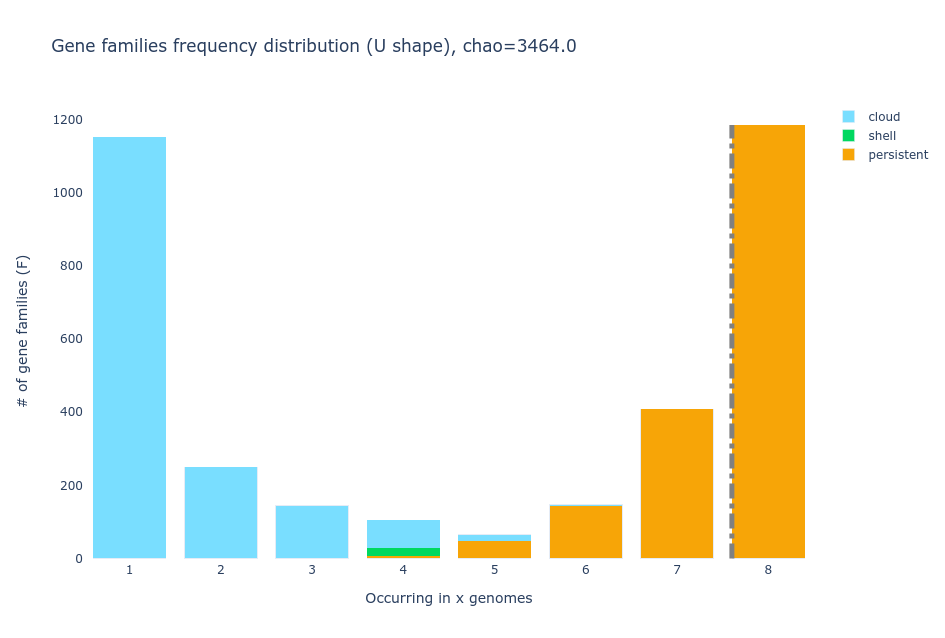
Genes : 16439
Organisms : 8
Families : 3464
Edges : 3887
Persistent ( min:0.5, max:1.0, sd:0.1, mean:0.94 ): 1793
Shell ( min:0.5, max:0.5, sd:0.0, mean:0.5 ): 22
Cloud ( min:0.12, max:0.75, sd:0.12, mean:0.19 ): 1649
Number of partitions : 3
If we want to have this in a file we can redirect this output adding > summary_statistics.txt to the command.
With the ppanggolin write command you can extract many text files and tables with a lot of information. For this, you need to provide the
pangenome.h5 file and the name of the directory to store the files. Each of the additional flags indicates which file or files to write. Let’s
use all of the flags that will give us basic information about our analysis. And then see what was generated.
$ ppanggolin write -p pangenome.h5 --output files --stats --csv --Rtab --partitions --projection --families_tsv
$ tree
.
├── files
│   ├── gene_families.tsv
│   ├── gene_presence_absence.Rtab
│   ├── matrix.csv
│   ├── mean_persistent_duplication.tsv
│   ├── organisms_statistics.tsv
│   ├── partitions
│   │   ├── cloud.txt
│   │   ├── exact_accessory.txt
│   │   ├── exact_core.txt
│   │   ├── persistent.txt
│   │   ├── shell.txt
│   │   ├── soft_accessory.txt
│   │   ├── soft_core.txt
│   │   ├── S.txt
│   │   └── undefined.txt
│   └── projection
│       ├── Streptococcus_agalactiae_18RS21_prokka.tsv
│       ├── Streptococcus_agalactiae_2603V_prokka.tsv
│       ├── Streptococcus_agalactiae_515_prokka.tsv
│       ├── Streptococcus_agalactiae_A909_prokka.tsv
│       ├── Streptococcus_agalactiae_CJB111_prokka.tsv
│       ├── Streptococcus_agalactiae_COH1_prokka.tsv
│       ├── Streptococcus_agalactiae_H36B_prokka.tsv
│       └── Streptococcus_agalactiae_NEM316_prokka.tsv
└── pangenome.h5
Exercise 1(Begginer): PPanGGolin results.
Go to small groups (if you are learning at a Workshop) and explore one result file or set of result files to see what information they are giving you. Then explain to the rest of the group what you learned.
Solution
gene_families.tsvis a table that shows you which individual genes (second column) correspond to which gene family (first column). It is the same as the one we provided with the GET_HOMOLOGUES results. When you don’t provide the clusters, PPanGGOLiN uses an algorithm that detects if a coding sequence appears to be a fragment, it uses this information to improve the clustering and it tells you which genes appear to be fragments in the third column of this file.gene_presence_absence.Rtabis a binary matrix that shows if a gene family is present (1) or absent (0) in each genome.matrix.csvis a table with one row per gene family, many columns with metadata, and one column per genome showing the name of the gene in the corresponding gene family.mean_persistent_duplication.tsvhas one row per persistent gene family and metrics about its duplication and if it is considered a single-copy marker.organisms_statistics.tsvhas one row per genome and columns for the number of gene families and genes in total and in each partition, the completeness and the number of single-copy markers.partitions/has one list per partition with the names of the gene families it contains.projection/has one file per genome with the metadata of each gene (i.e. contig, coordinates, strand, gene family, number of copies, partition, neighbors in each partition).
Draw interactive plots
We can also extract two interactive plots with the command ppanggolin draw, following a similar syntax as with the command ppanggolin write.
$ ppanggolin draw --pangenome pangenome.h5 --output plots --ucurve --tile_plot
$ tree plots/
plots/
├── tile_plot.html
└── Ushaped_plot.html
Let’s download them to our local machines to explore them. Open a new local terminal, navigate to the directory where you want the files
and use the scp command.
$ scp -r user@server-address:~/pan_workshop/results/pangenome/ppanggolin/pangenome/plots .
Open both html files in a browser and explore them. They are interactive so play with the plots for a while to see what information can be
obtained from them.
- U-shaped plot
The U-shaped plot is a bar chart where you can see how many gene families (y-axis) are in how many genomes (x-axis). They are colored according to the
partition they belong to.
- Tile plot
The tile plot is a presence/absence heatmap of the gene families (y-axis) in each genome (x-axis) ordered by hierarchical clustering and showing the
multicopy families.
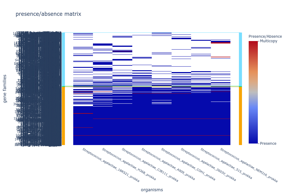
Difficulty showing the plots?
If your browser is taking too long to open your tile plot repeat the
pangolin drawcommand with the option--nocloud, this will remove the families in the cloud partition from the plot to make it easier to handle.
Discussion: Partitions
Why are there bars with two partitions in the U plot?
Solution
Because in PPanGGOLiN the partitions not only depend on the number of genomes a gene family is present in but also on the conservation of the neighborhood of the gene. For example, a gene that is in only a few genomes but has the same shell neighbors in all or most of them, will more likely be placed in the shell than in the cloud.
Draw the pangenome graph
Now it’s time to see the actual partitioned graph. For that, we can use the ppanggolin write command.
$ ppanggolin write -p pangenome.h5 --gexf --output gexf
Let’s download the gexf file to our local machines to explore it. Open a new local terminal, navigate to the directory where you want the file
and use the scp command.
$ scp -r user@server-address:~/pan_workshop/results/pangenome/ppanggolin/pangenome/gexf .
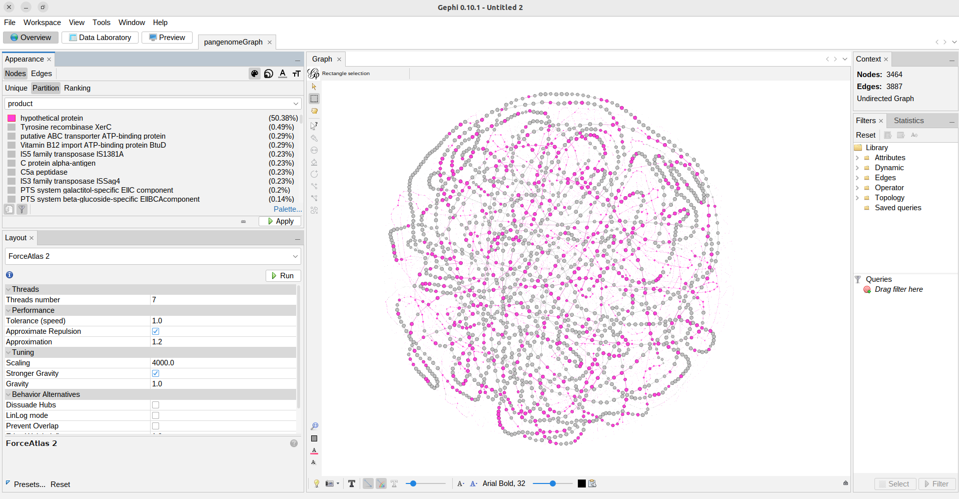
To view the interactive graph we will use the software gephi.
Gephi setup
Download from this web page the gephi installer that suits your opperating system.
Open gephi:
Linux
Go to the directory where you downloaded the program and type:
$ ./gephi-0.10.1/bin/gephiIf you do not see the graph properly you may have problems with the video driver. Open it this way instead:
$ LIBGL_ALWAYS_SOFTWARE=1 ./gephi-0.10.1/bin/gephiWindows and Mac
Click the Gephi icon to open the App.
If your download is in a language that is not English, change the language to English to make it easier to find the options that we will mention. Find the equivalent to
Tools/Language/Englishin the top left menu and restart gephi.
Steps to see the graph in gephi
1) Go to File/Open/and select the file pangenomeGraph.gexf.
2) Click OK in the window that appears.
3) Scroll out with your mouse.
4) Go to the Layout section on the left and in the selection bar choose ForceAtlas2.
5) In the Tuning section change the Scaling value to 4000 and check the Stronger Gravity box.
6) Click on the Run button and then click it again to stop.
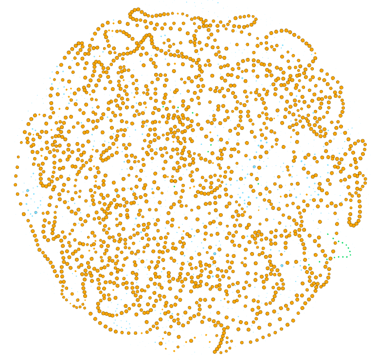
Now we have a pangenome graph!
Exercise 2(Intermediate): Exploring the pangenome graph.
Finally we are looking at the pangenome graph. Here each node is a gene family, if you click on the black T at the bottom of the graph you can label them.
Explore the options of visualization for the pangenome graph, while trying to identify what each element of the graph represents (i.e. size of nodes and edges, etc.) and what is in the Data Laboratory.
Use the Appearance section to color the nodes and edges according to the attributes that you find most useful, like:
a) Partition.
b) Number of organisms.
c) Number of genes.
d) Product.
Solution
In the top left panel you can color the nodes or edges according to different data. You can choose discrete palettes in the partition section and gradients in the Ranking section. You can choose the palette, generate a new one, or choose colors one by one.
a) Nodes colored according to the partition they belong to.
b) Nodes colored according to the number of organisms they are present in.
c) Nodes colored according to the number of genes that are part of the family.
d) nodes colored according to the protein function,
Special analyses
Besides being able to work with thousands of genomes and having the approach of the partitioned graph, PPanGGOLiN is unique in that it allows you to analyze your pangenomes in different ways. You can obtain the Regions of Genome Plasticity (RGP) of your pangenomes, which are stretches of shell and cloud genes, and the location in the pangenome where many genomes have an RGP, which are called Spots of Insertion.
You can also use PPanGGOLiN to identify Conserved Modules, groups of accessory genes that are usually together and may be functional modules. And you can find the modules present in RGPs and Spots of Insertion.
To see how your pangenome grows as more genomes are added and know if it is open or closed you can do Rarefaction analysis.
If you are interested in the phylogeny of your genomes, you can retrieve the Multiple Sequence Alignment of each gene family and a concatenation of all single-copy exact core genes.
These analyses, and more, can be done by using commands that enrich your pangenome.h5 file and extracting the appropriate outputs with the ppanggolin write command. Check the PPanGGOLiN Wiki to learn how to perform them.
References:
Go to the PPanGGOLiN GitHub Wiki for the complete collection of instructions and posibilities.
And read the original PPanGGOLiN article to understand the details:Gautreau G et al. (2020) PPanGGOLiN: Depicting microbial diversity via a partitioned pangenome graph. PLOS Computational Biology 16(3): e1007732. https://doi.org/10.1371/journal.pcbi.1007732.
Key Points
PPanGGOLiN is a software to create and manipulate prokaryotic pangenomes.
PPanGGOLiN integrates gene families and their genomic neighborhood to build a graph and define the partitions.
PPanGGOLiN is designed to scale up to tens of thousands of genomes.