Overview

Teaching: 45 min
Exercises: 15 min

Questions

• How do I perform data transformations such as removing columns on my data using R?

• What are tidy data (in opposition to messy data)?

• How do I import data into R (e.g. from a web link)?

• How can I make my code more readable when performing a series of transformation?

Objectives

• Learn how to explore a publically available dataset (gapminder).

• Learn how to perform data transformation with the dplyr functions from the tidyverse package

Table of contents

• 1. Introduction
  • 1.1 Why should we care about data transformation?
  • 1.2 Gapminder dataset
  • 1.3 Load the tidyverse suite
  • 1.4 Create a new R Markdown file.
• 2. Explore the gapminder dataframe
  • 2.1 Import data with readr::read_csv()
  • 2.2 Dataset inspection
  • 2.3 Descriptive statistics of the gapminder dataset
• 3. dplyr basics
  • 3.1 filter() observations
  • 3.2 select() variables
  • 3.3 The pipe %>% operator
  • 3.4 mutate() adds new variables
  • 3.5 group_by makes group that can be summarize()
  • 3.6 arrange() orders columns
• 4. All together now
  • 4.1 With dplyr
  • 4.2 With base R
• 5. Joining datasets
  • 5.1 Types of join
  • 5.2 Join the gapminder dataset with a co2 dataset
• 6. Resources and credits

1. Introduction

1.1 Why should we care about data transformation?

Data scientists, according to interviews and expert estimates, spend from 50 percent to 80 percent of their time mired in the mundane labor of collecting and preparing data, before it can be explored for useful information. - NYTimes (2014)

What are some common things you like to do with your data? Maybe remove rows or columns, do calculations and maybe add new columns? This is called data wrangling (or more simply data transformation). It’s not data management or data manipulation: you keep the raw data raw and do these things programatically in R with the tidyverse.

We are going to introduce you to data wrangling in R first with the tidyverse. The tidyverse is a new suite of packages that match a philosophy of data science developed by Hadley Wickham and the RStudio team. I find it to be a more straight-forward way to learn R. We will also show you by comparison what code will look like in base-R, which means, in R without any additional packages (like the tidyverse package) installed. I like David Robinson’s blog post on the topic of teaching the tidyverse first.

For some things, base-R is more straightforward, and we’ll show you that too. Whenever we use a function that is from the tidyverse, we will prefix it so you’ll know for sure.

1.2 Gapminder dataset

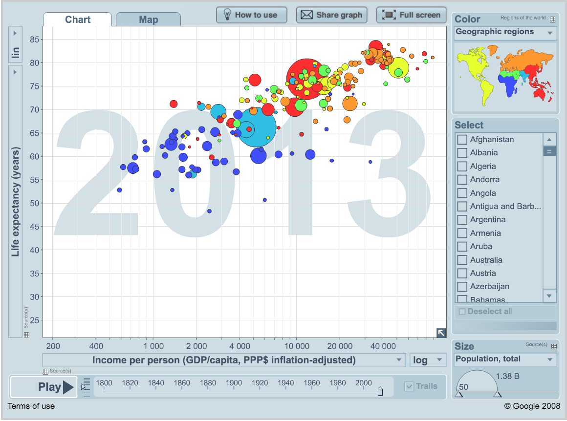
We’ll be using Gapminder data, which represents the health and wealth of nations. It was pioneered by Hans Rosling, who is famous for describing the prosperity of nations over time through famines, wars and other historic events with this beautiful data visualization in his 2006 TED Talk: The best stats you’ve ever seen:

1.3 Load the tidyverse suite

We’ll use the package dplyr, which is bundled within the tidyverse suite of packages. Please load the tidyverse if not already done.

library("tidyverse")

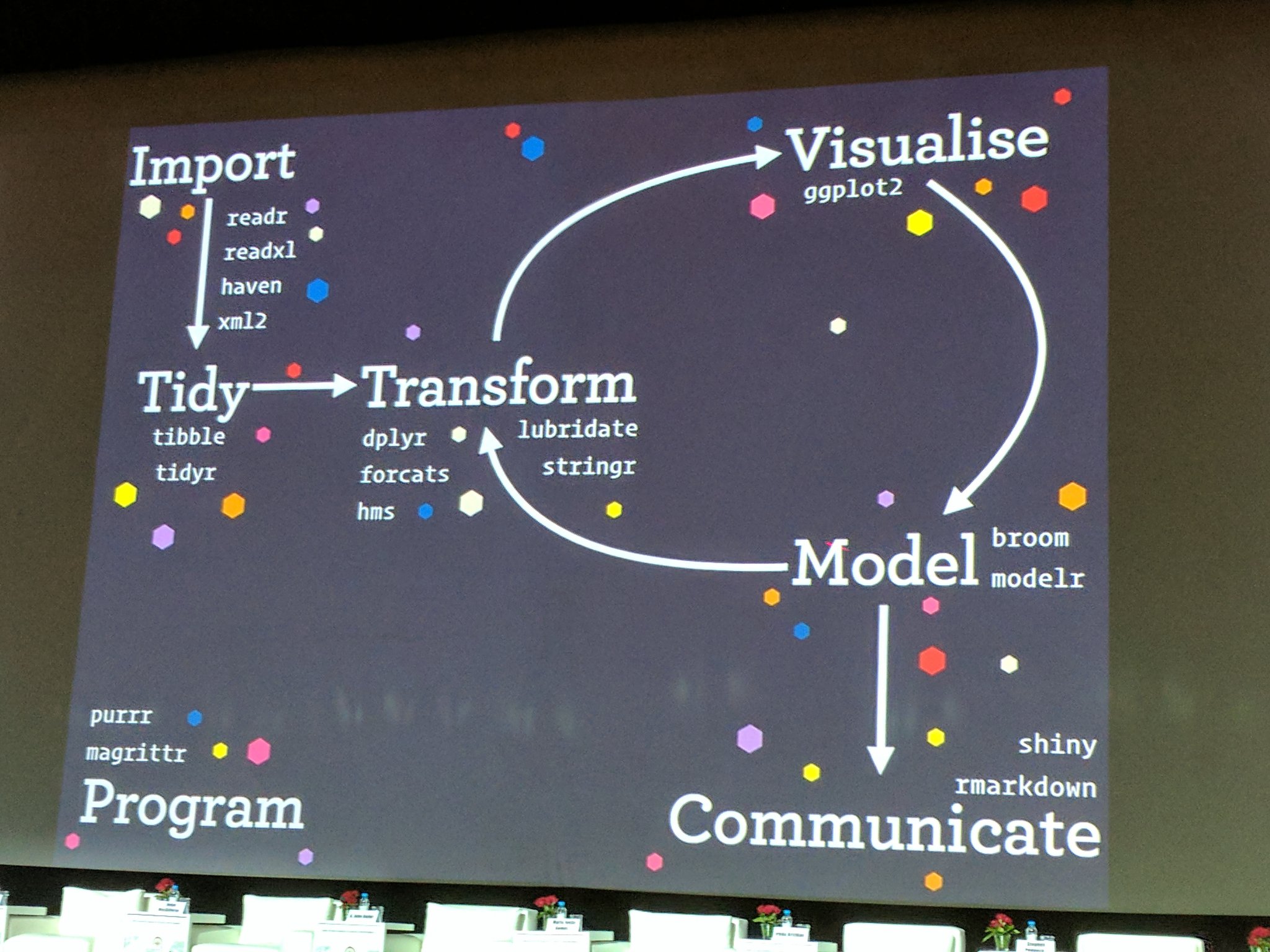
The tidyverse package suite contains all the tools you need for data science. Actually, Hadley Wickham and RStudio have created a ton of packages that help you at every step of the way here. This is from one of Hadley’s presentations:

1.4 Create a new R Markdown file.

We’ll do this in a new R Markdown file.

Here’s what to do:

1. Clear your workspace (Session > Restart R)
2. New File > R Markdown…
3. Save as gapminder-wrangle.Rmd
4. Delete the irrelevant text and write a little note to yourself about this section: “cleaning and transforming the gapminder dataset.”

2. Explore the gapminder dataframe

Previously, we explored the national parks dataframe visually. Today, we’ll explore a dataset by the numbers. We will work with some of the data from the Gapminder project.

The data are on GitHub. Navigate to: https://github.com/carpentries-incubator/open-science-with-r/blob/gh-pages/data/gapminder.csv.

This is data-view mode: so we can have a quick look at the data. It’s a .csv file, which you’ve probably encountered before, but GitHub has formatted it nicely so it’s easy to look at. You can see that for every country and year, there are several columns with data in them.

2.1 Import data with readr::read_csv()

We can read this data into R directly from GitHub, without downloading it. But we can’t read this data in view-mode. We have to click on the Raw button on the top-right of the data. This displays it as the raw csv file, without formatting.

Copy the url for raw data: https://raw.githubusercontent.com/carpentries-incubator/open-science-with-r/gh-pages/data/gapminder.csv

Now, let’s go back to RStudio. In our R Markdown, let’s read this .csv file and name the variable gapminder. We will use the read_csv() function from the readr package (part of the tidyverse, so it’s already installed!).

## read gapminder csv. Note the readr:: prefix identifies which package it's in
gapminder <- readr::read_csv('https://raw.githubusercontent.com/carpentries-incubator/open-science-with-r/gh-pages/data/gapminder.csv') 

Note

read_csv works with local filepaths as well, you could use one from your computer.

2.2 Dataset inspection

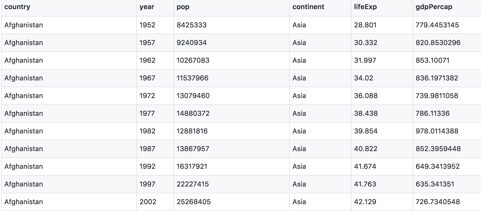
Let’s inspect the data with head and tail:

head(gapminder) # shows first 6
tail(gapminder) # shows last 6

head(gapminder, n = 10) # shows first X that you indicate
tail(gapminder, n = 12) # guess what this does!

str() will provide a sensible description of almost anything: when in doubt, inspect using str() on some of the recently created objects to get some ideas about what to do next.

str(gapminder) # ?str - displays the structure of an object

 str(gapminder)
Classes ‘spec_tbl_df’, ‘tbl_df’, ‘tbl’ and 'data.frame':	1704 obs. of  6 variables:
 $ country  : chr  "Afghanistan" "Afghanistan" "Afghanistan" "Afghanistan" ...
 $ year     : num  1952 1957 1962 1967 1972 ...
 $ pop      : num  8425333 9240934 10267083 11537966 13079460 ...
 $ continent: chr  "Asia" "Asia" "Asia" "Asia" ...
 $ lifeExp  : num  28.8 30.3 32 34 36.1 ...
 $ gdpPercap: num  779 821 853 836 740 ...
 - attr(*, "spec")=
  .. cols(
  ..   country = col_character(),
  ..   year = col_double(),
  ..   pop = col_double(),
  ..   continent = col_character(),
  ..   lifeExp = col_double(),
  ..   gdpPercap = col_double()
  .. )

This will show how R understood your data types. Check that numbers are indeed understood as num/numeric and strings as chr/character.

You can get the number of rows and columns of the gapminder dataframe with dim().

dim(gapminder)

[1] 1704    6

It shows that our dataframe has 1704 rows and 6 columns.

R imports gapminder as a dataframe. We aren’t going to get into the other types of data receptacles today (‘arrays’, ‘matrices’), because working with dataframes is what you should primarily use. Why?

• dataframes contain related variables neatly together, great for analysis
• most functions, including the latest and greatest packages actually require that your data be in a dataframe
• dataframes can hold variables of different flavors such as:
  • character data (country or continent names; “Characters (chr)”)
  • quantitative data (years, population; “Integers (int)” or “Numeric (num)”)
  • categorical information (male vs. female)

We can also see the gapminder variable in RStudio’s Environment pane (top right).

More ways to learn basic info on a dataframe.

names(gapminder)  # column names
ncol(gapminder)   # ?ncol number of columns
nrow(gapminder)   # ?nrow number of rows

2.3 Descriptive statistics of the gapminder dataset

A statistical overview can be obtained with summary(), or with skimr::skim()

summary(gapminder)

   country               year           pop             continent            lifeExp        gdpPercap       
 Length:1704        Min.   :1952   Min.   :6.001e+04   Length:1704        Min.   :23.60   Min.   :   241.2  
 Class :character   1st Qu.:1966   1st Qu.:2.794e+06   Class :character   1st Qu.:48.20   1st Qu.:  1202.1  
 Mode  :character   Median :1980   Median :7.024e+06   Mode  :character   Median :60.71   Median :  3531.8  
                    Mean   :1980   Mean   :2.960e+07                      Mean   :59.47   Mean   :  7215.3  
                    3rd Qu.:1993   3rd Qu.:1.959e+07                      3rd Qu.:70.85   3rd Qu.:  9325.5  
                    Max.   :2007   Max.   :1.319e+09                      Max.   :82.60   Max.   :113523.1  

This will give simple descriptive statistics (e.g. median, average) for each column if numeric.

Finally, the skimr package provides a powerful descriptive function for dataframes.

library(skimr) 
skim(gapminder)

── Data Summary ────────────────────────
                           Values   
Name                       gapminder
Number of rows             1704     
Number of columns          6        
_______________________             
Column type frequency:              
  character                2        
  numeric                  4        
________________________            
Group variables            None     

── Variable type: character ──────────────────────────────────────────────────────────────────────────────────────────────────────────────
  skim_variable n_missing complete_rate   min   max empty n_unique whitespace
1 country               0             1     4    24     0      142          0
2 continent             0             1     4     8     0        5          0

── Variable type: numeric ────────────────────────────────────────────────────────────────────────────────────────────────────────────────
  skim_variable n_missing complete_rate       mean          sd      p0       p25       p50        p75         p100 hist 
1 year                  0             1     1980.         17.3  1952      1966.     1980.      1993.        2007   ▇▅▅▅▇
2 pop                   0             1 29601212.  106157897.  60011   2793664   7023596.  19585222.  1318683096   ▇▁▁▁▁
3 lifeExp               0             1       59.5        12.9    23.6      48.2      60.7       70.8         82.6 ▁▆▇▇▇
4 gdpPercap             0             1     7215.       9857.    241.     1202.     3532.      9325.      113523.  ▇▁▁▁▁

This gives you a comprehensive view of your data at a glance.

3. dplyr basics

OK, so let’s start wrangling with the dplyr collection of functions. .

There are five dplyr functions that you will use to do the vast majority of data manipulations:

• filter(): pick observations by their values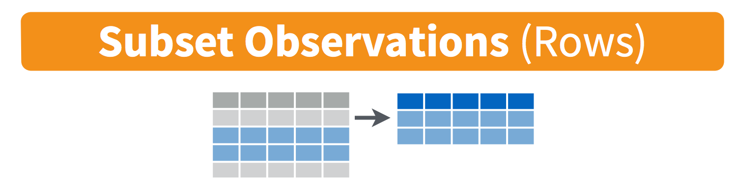

  

• select(): pick variables by their names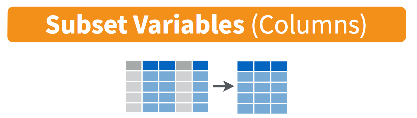

  

• mutate(): create new variables with functions of existing variables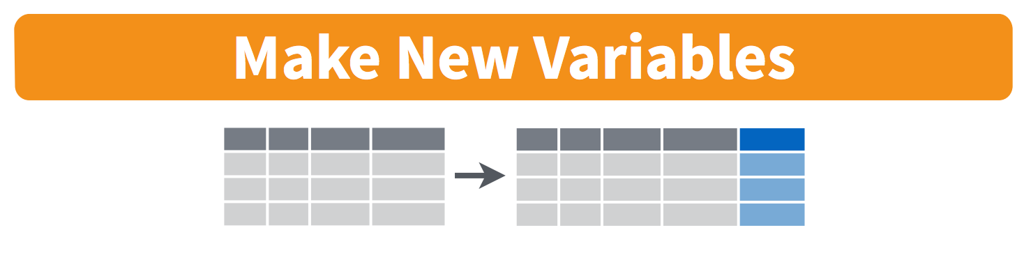

  

• summarise(): collapse many values down to a single summary

  

• arrange(): reorder the rows

These can all be used in conjunction with group_by() which changes the scope of each function from operating on the entire dataset to operating on it group-by-group. These six functions provide the verbs for a language of data manipulation.

All verbs work similarly:

1. The first argument is a data frame.
2. The subsequent arguments describe what to do with the data frame. You can refer to columns in the data frame directly without using $.
3. The result is a new data frame.

Together these properties make it easy to chain together multiple simple steps to achieve a complex result.

3.1 filter() observations

You will want to isolate bits of your data; maybe you want to only look at a single country or a few years. R calls this subsetting.

filter() is a function in dplyr that takes logical expressions and returns the rows for which all are TRUE.

Visually, we are doing this:

Remember your logical expressions from this morning? We’ll use < and == here.

filter(gapminder, lifeExp < 29)

You can say this out loud: “Filter the gapminder data for life expectancy less than 29”. Notice that when we do this, all the columns are returned, but only the rows that have the life expectancy less than 29. We’ve subsetted by row.

Let’s try another: “Filter the gapminder data for the country Mexico”.

filter(gapminder, country == "Mexico")

How about if we want two country names? We can’t use the == operator here, because it can only operate on one thing at a time. We will use the %in% operator:

filter(gapminder, country %in% c("Mexico", "Peru"))

How about if we want Mexico in 2002? You can pass filter different criteria:

filter(gapminder, country == "Mexico", year == 2002)

Exercise

What is the mean life expectancy of Sweden?
Hint: do this in 2 steps by assigning a variable and then using the mean() function.

Solution

sweden <- filter(gapminder, country == "Sweden")
mean(sweden$lifeExp)

3.2 select() variables

We use select() to subset the data on variables or columns.

Visually, we are doing this:

We can select multiple columns with a comma, after we specify the data frame (gapminder).

select(gapminder, year, lifeExp) 

We can also use - to deselect columns

select(gapminder, -continent, -lifeExp) # you can use - to deselect columns

3.3 The pipe %>% operator

What if we want to use select() and filter() together?

Let’s filter for Cambodia and remove the continent and lifeExp columns. We’ll save this as a variable. Actually, as two temporary variables, which means that for the second one we need to operate on gap_cambodia, not gapminder.

gap_cambodia  <- filter(gapminder, country == "Cambodia")
gap_cambodia2 <- select(gap_cambodia, -continent, -lifeExp) 

We also could have called them both gap_cambodia and overwritten the first assignment. Either way, naming them and keeping track of them gets super cumbersome, which means more time to understand what’s going on and opportunities for confusion or error.

Good thing there is an awesome alternative.

Before we go any further, we should exploit the new pipe operator that comes from the magrittr package by Stefan Bache. The package name refers to the Belgium surrealist artist René Magritte that made a famous painting with a pipe.

The %>% operator is going to change your life. You no longer need to enact multi-operation commands by nesting them inside each other. And we won’t need to make temporary variables like we did in the Cambodia example above. This new syntax leads to code that is much easier to write and to read: it actually tells the story of your analysis.

Here’s what it looks like: %>%.

Keyboard shortcuts for the pipe operator

The RStudio keyboard shortcut: Ctrl + Shift + M (Windows), Cmd + Shift + M (Mac).

Let’s demo then I’ll explain:

gapminder %>% head()

# A tibble: 6 x 6
  country      year      pop continent lifeExp gdpPercap
  <chr>       <dbl>    <dbl> <chr>       <dbl>     <dbl>
1 Afghanistan  1952  8425333 Asia         28.8      779.
2 Afghanistan  1957  9240934 Asia         30.3      821.
3 Afghanistan  1962 10267083 Asia         32.0      853.
4 Afghanistan  1967 11537966 Asia         34.0      836.
5 Afghanistan  1972 13079460 Asia         36.1      740.
6 Afghanistan  1977 14880372 Asia         38.4      786.

This is equivalent to head(gapminder).
This pipe operator takes the thing on the left-hand-side and pipes it into the function call on the right-hand-side. It literally drops it in as the first argument.

Never fear, you can still specify other arguments to this function! To see the first 3 rows of Gapminder, we could say head(gapminder, n = 3) or this:

gapminder %>% head(n = 3)

I’ve advised you to think “gets” whenever you see the assignment operator, <-. Similarly, you should think “and then” whenever you see the pipe operator, %>%.

One of the most awesome things about this is that you START with the data before you say what you’re doing to DO to it. So above: “take the gapminder data, and then give me the first three entries”.

This means that instead of this:

## instead of this...
gap_cambodia  <- filter(gapminder, country == "Cambodia")
gap_cambodia2 <- select(gap_cambodia, -continent, -lifeExp) 

## ...we can do this
gap_cambodia  <- gapminder %>% filter(country == "Cambodia")
gap_cambodia2 <- gap_cambodia %>% select(-continent, -lifeExp) 

So you can see that we’ll start with gapminder in the first example line, and then gap_cambodia in the second. This makes it a bit easier to see what data we are starting with and what we are doing to it.

Exercise

Can you filter for Finland and show only the pop (population) column?
Use the pipe %>% operator twice.

Solution

gapminder %>% filter(country == "Finland") %>% select(pop)

We can use the pipe to chain those two operations together:

gap_cambodia  <- gapminder %>% filter(country == "Cambodia") %>%
  select(-continent, -lifeExp) 

What’s happening here? In the second line, we were able to delete gap_cambodia2 <- gap_cambodia, and put the pipe operator above. This is possible since we wanted to operate on the gap_cambodia data anyways. And we weren’t truly excited about having a second variable named gap_cambodia2 anyways, so we can get rid of it. This is huge, because most of your data wrangling will have many more than 2 steps, and we don’t want a gap_cambodia14!

Let’s write it again but using multiple lines so it’s nicer to read.

gap_cambodia  <- gapminder %>% 
  filter(country == "Cambodia") %>%
  select(-continent, -lifeExp) 

Amazing. I can actually read this like a story and there aren’t temporary variables that get super confusing. In my head:

start with the gapminder data, and then
filter for Cambodia, and then
deselect the variables continent and lifeExp.

Being able to read a story out of code like this is really game-changing. We’ll continue using this syntax as we learn the other dplyr verbs.

3.4 mutate() adds new variables

Alright, let’s keep going.

Let’s say we need to compute a new variable from two pre-existing variables in the dataframe. We could calculate the Gross Domestic Product from the gdpPercap (GDP per person) and the pop (population) variables.

Visually, we are doing this:

We will name our new column gdp and assign it with a single =.

gapminder %>%
  mutate(gdp = pop * gdpPercap)

   country      year      pop continent lifeExp gdpPercap          gdp
   <chr>       <dbl>    <dbl> <chr>       <dbl>     <dbl>        <dbl>
 1 Afghanistan  1952  8425333 Asia         28.8      779.  6567086330.
 2 Afghanistan  1957  9240934 Asia         30.3      821.  7585448670.
 3 Afghanistan  1962 10267083 Asia         32.0      853.  8758855797.
 4 Afghanistan  1967 11537966 Asia         34.0      836.  9648014150.
 5 Afghanistan  1972 13079460 Asia         36.1      740.  9678553274.
 6 Afghanistan  1977 14880372 Asia         38.4      786. 11697659231.
 7 Afghanistan  1982 12881816 Asia         39.9      978. 12598563401.
 8 Afghanistan  1987 13867957 Asia         40.8      852. 11820990309.
 9 Afghanistan  1992 16317921 Asia         41.7      649. 10595901589.
10 Afghanistan  1997 22227415 Asia         41.8      635. 14121995875.

This is quite handy when you need to calculate a percentage for example.

Exercise

Find the maximum gdpPercap of Egypt and the maximum gdpPercap of Vietnam. Create a new column with mutate().
Hint: use max().

Solution

Egypt:
gapminder %>%
select(-continent, -lifeExp) %>% (not super necessary but to simplify)
filter(country == "Egypt") %>%
mutate(gdp = pop * gdpPercap) %>%
mutate(max_gdp = max(gdp))

Vietnam:
gapminder %>%
select(-continent, -lifeExp) %>% (not super necessary but to simplify)
filter(country == "Vietnam") %>%
mutate(gdp = pop * gdpPercap, max_gdp = max(gdp)) (multiple variables created)

With the things we know so far, the answers you have are maybe a bit limiting. First, we had to act on Egypt and Vietnam separately, and repeat the same code. Copy-pasting like this is also super error prone.

And second, this max_gdpPercap column is pretty redundant, because it’s a repeated value a ton of times. Sometimes this is exactly what you want! You are now set up nicely to maybe take a proportion of gdpPercap/max_gdpPercap for each year or something. But maybe you only wanted that max_gdpPercap for something else. Let’s keep going…

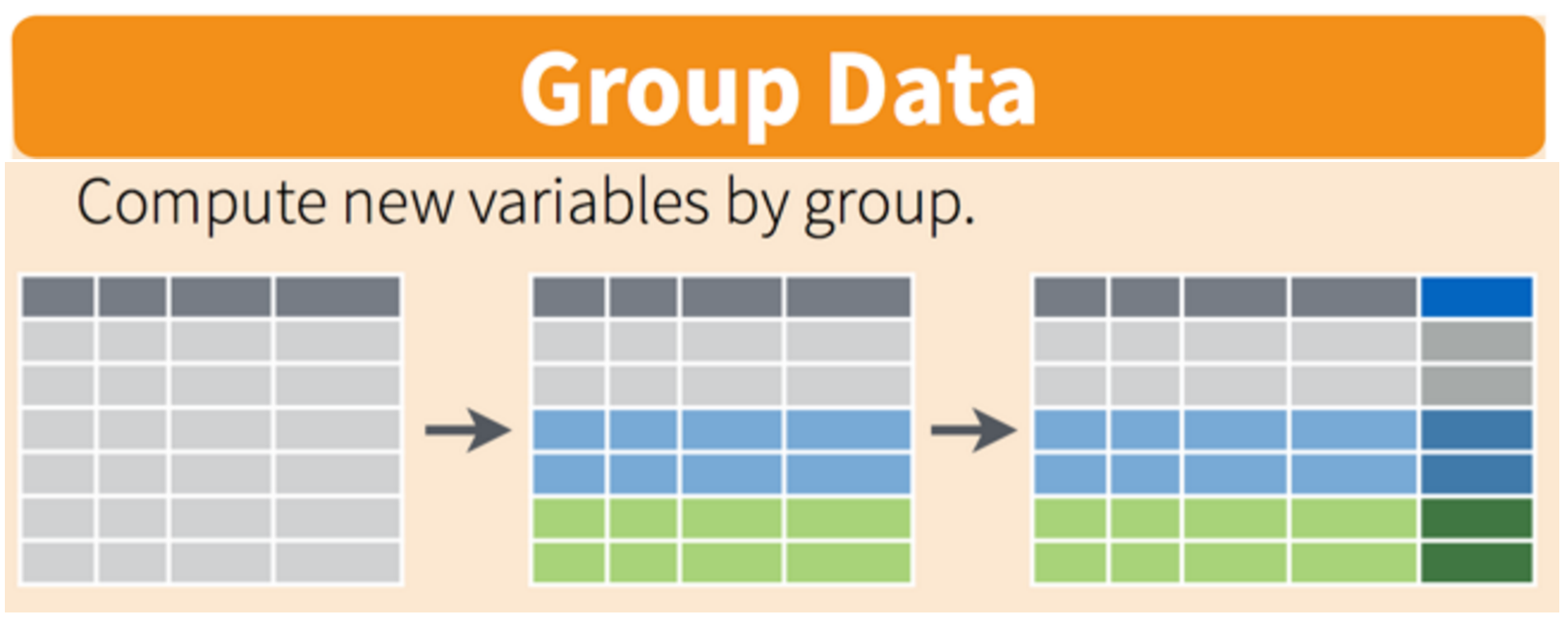
3.5 group_by makes group that can be summarize()

group_by operates on groups

Let’s tackle that first issue first. So how do we less painfully calculate the max gdpPercap for all countries?

Visually, we are doing this:

gapminder %>%
  group_by(country) %>%
  mutate(gdp = pop * gdpPercap, max_gdp = max(gdp)) %>%
  ungroup() # if you use group_by, also use ungroup() to save heartache later

The ungroup() serves to allow operations again (mutate or summarize) on the grouping variables. If you would like to change something on country you would need to ungroup() them first. For an extensive discussion about ungroup, see the RStudio community forum here.

So instead of filtering for a specific country, we’ve grouped by country, and then done the same operations. It’s hard to see; let’s look at a bunch at the tail:

gapminder %>%
  group_by(country) %>%
  mutate(gdp = pop * gdpPercap, 
  	     max_gdp = max(gdp)) %>%
  ungroup() %>% 
  tail(30)

 country     year      pop continent lifeExp gdpPercap          gdp      max_gdp
   <chr>      <dbl>    <dbl> <chr>       <dbl>     <dbl>        <dbl>        <dbl>
 1 Yemen Rep.  1982  9657618 Asia         49.1     1978. 19098490176. 50659874994.
 2 Yemen Rep.  1987 11219340 Asia         52.9     1972. 22121638707. 50659874994.
 3 Yemen Rep.  1992 13367997 Asia         55.6     1879. 25125105886. 50659874994.
 4 Yemen Rep.  1997 15826497 Asia         58.0     2117. 33512362498. 50659874994.
 5 Yemen Rep.  2002 18701257 Asia         60.3     2235. 41793958635. 50659874994.
 6 Yemen Rep.  2007 22211743 Asia         62.7     2281. 50659874994. 50659874994.
 7 Zambia      1952  2672000 Africa       42.0     1147.  3065822956. 14931695864.
 8 Zambia      1957  3016000 Africa       44.1     1312.  3956861606. 14931695864.
 9 Zambia      1962  3421000 Africa       46.0     1453.  4969774845. 14931695864.
10 Zambia      1967  3900000 Africa       47.8     1777.  6930601540. 14931695864.

OK, this is great. But what if this what we needed, a max_gdp value for each country. We don’t need that kind of repeated value for each of the max_gdp values. Here’s the next function:

summarize() compiles values for each group

We want to operate on a group, but actually collapse or distill the output from that group. The summarize() function will do that for us.

Visually, we are doing this:

Here we go:

gapminder %>%
  group_by(country) %>%
  mutate(gdp = pop * gdpPercap) %>%
  summarize(max_gdp = max(gdp)) %>%
  ungroup()

  country           max_gdp
   <chr>               <dbl>
 1 Afghanistan  31079291949.
 2 Albania      21376411360.
 3 Algeria     207444851958.
 4 Angola       59583895818.
 5 Argentina   515033625357.
 6 Australia   703658358894.
 7 Austria     296229400691.
 8 Bahrain      21112675360.
 9 Bangladesh  209311822134.
10 Belgium     350141166520.

How cool is that! summarize() will actually only keep the columns that are grouped_by or summarized. So if we wanted to keep other columns, we’d have to do have a few more steps.

3.6 arrange() orders columns

This is ordered alphabetically, which is cool. But let’s say we wanted to order it in ascending order for max_gdp. The dplyr function is arrange().

gapminder %>%
  group_by(country) %>%
  mutate(gdp = pop * gdpPercap) %>%
  summarize(max_gdp = max(gdp)) %>%
  ungroup() %>%
  arrange(max_gdp)

   country                      max_gdp
   <chr>                          <dbl>
 1 Sao Tome and Principe     319014077.
 2 Comoros                   701111696.
 3 Guinea-Bissau             950984749.
 4 Djibouti                 1033689705.
 5 Gambia                   1270911775.
 6 Liberia                  1495937378.
 7 Central African Republic 3084613079.
 8 Lesotho                  3158513357.
 9 Burundi                  3669693671.
10 Eritrea                  3707155863.

Your turn

Exercise

1. Arrange your data frame in descending order (opposite of what we’ve done). Look at the documentation ?arrange
2. Find the maximum life expectancy for countries in Asia. What is the earliest year you encounter? The latest? Hint: you can use either base::max or dplyr::arrange()…

Solution

1) arrange(desc(max_gdp)) 2) gapminder %>% filter(continent == 'Asia') %>% group_by(country) %>% filter(lifeExp == max(lifeExp)) %>% arrange(year)

4. All together now

We have done a pretty incredible amount of work in a few lines. Our whole analysis is this. Imagine the possibilities from here. It’s very readable: you see the data as the first thing, it’s not nested. Then, you can read the verbs. This is the whole thing, with explicit package calls from readr:: and dplyr::

4.1 With dplyr

# load libraries
library(tidyverse) 

# read in data
gapminder <- readr::read_csv('https://raw.githubusercontent.com/carpentries-incubator/open-science-with-r/gh-pages/data/gapminder.csv') 

## summarize
gap_max_gdp <- gapminder %>% 
  dplyr::select(-continent, -lifeExp) %>% # or select(country, year, pop, gdpPercap)
  dplyr::group_by(country) %>%
  dplyr::mutate(gdp = pop * gdpPercap) %>%
  dplyr::summarize(max_gdp = max(gdp)) %>%
  dplyr::ungroup() 

I actually am borrowing this “All together now” from Tony Fischetti’s blog post How dplyr replaced my most common R idioms. With that as inspiration, this is how what we have done would look like in Base R.

4.2 With base R

Let’s compare with some base R code to accomplish the same things. Base R requires subsetting with the [rows, columns] notation. This notation is something you’ll see a lot in base R. the brackets [ ] allow you to extract parts of an object. Within the brackets, the comma separates rows from columns.

If we don’t write anything after the comma, that means “all columns”. And if we don’t write anything before the comma, that means “all rows”.

Also, the $ operator is how you access specific columns of your dataframe. You can also add new columns like we will do with mex$gdp below.

Instead of calculating the max for each country like we did with dplyr above, here we will calculate the max for one country, Mexico. Tomorrow we will learn how to do it for all the countries, like we did with dplyr::group_by().

## gapminder-wrangle.R --- baseR
## J. Lowndes lowndes@nceas.ucsb.edu

gapminder <- read.csv('https://raw.githubusercontent.com/carpentries-incubator/open-science-with-r/gh-pages/data/gapminder.csv', stringsAsFactors = FALSE) 
x1  <- gapminder[ , c('country', 'year', 'pop', 'gdpPercap') ] # subset columns
mex <- x1[x1$country == "Mexico", ] # subset rows
mex$gdp <- mex$pop * mex$gdpPercap # add new columns
mex$max_gdp <- max(mex$gdp)

Note too that the chain operator %>% that we used with the tidyverse lets us get away from the temporary variable x1.

Discussion

What do you personally favor? What are pros and cons of the dplyr and base methods?
Both dplyr and base solutions are fine. In the long run, you might better understand the pros and cons of each method.

5. Joining datasets

We’ve learned a ton in this session and we may not get to this right now. If we don’t have time, we’ll start here before getting into the next chapter: tidyr.

5.1 Types of join

Most of the time you will have data coming from different places or in different files, and you want to put them together so you can analyze them. Datasets you’ll be joining can be called relational data, because it has some kind of relationship between them that you’ll be acting upon. In the tidyverse, combining data that has a relationship is called “joining”.

From the RStudio cheatsheet (note: this is an earlier version of the cheatsheet but I like the graphics):

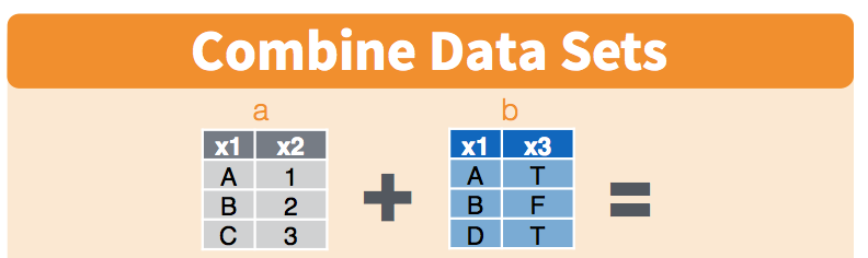
Let’s have a look at this and pretend that the x1 column is a study site and x2 is the variables we’ve recorded (like species count) and x3 is data from an instrument (like temperature data). Notice how you may not have exactly the same observations in the two datasets: in the x1 column, observations A and B appear in both datasets, but notice how the table on the left has observation C, and the table on the right has observation D.

If you wanted to combine these two tables, how would you do it? There are some decisions you’d have to make about what was important to you. The cheatsheet visualizes it for us:

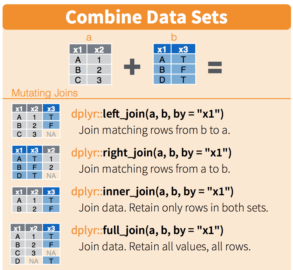
We will only talk about this briefly here, but you can refer to this more as you have your own datasets that you want to join. This describes the figure above::

• left_join keeps everything from the left table and matches as much as it can from the right table. In R, the first thing that you type will be the left table (because it’s on the left)
• right_join keeps everything from the right table and matches as much as it can from the left table
• inner_join only keeps the observations that are similar between the two tables
• full_join keeps all observations from both tables.

I like graphical representations of complex things so here’s a nice one taken from a blog post:

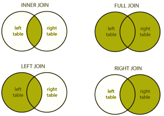
You can visualise the different outputs from the different joins.

5.2 Join the gapminder dataset with a co2 dataset

Let’s play with these CO2 emissions data to illustrate:

## read in the data.
co2 <- read_csv("https://raw.githubusercontent.com/carpentries-incubator/open-science-with-r/gh-pages/data/co2.csv")

## explore
co2 %>% head()

# A tibble: 6 x 2
  country        co2_2007
  <chr>             <dbl>
1 Afghanistan      2938. 
2 Albania          4218. 
3 Algeria        105838. 
4 American Samoa     18.4
5 Angola          17405. 
6 Anguilla           12.4

It is a simple dataframe with countries and their level of CO2 in 2007.

Let’s filter the gapminder dataset for the year 2007.

## create new variable that is only 2007 data
gap_2007 <- gapminder %>%
  filter(year == 2007) 

## left_join gap_2007 to co2
gapminder_with_co2_left <- left_join(gap_2007, co2, by = "country")

## First lines
gapminder_with_co2_left

  country      year       pop continent lifeExp gdpPercap co2_2007
   <chr>       <dbl>     <dbl> <chr>       <dbl>     <dbl>    <dbl>
 1 Afghanistan  2007  31889923 Asia         43.8      975.    2938.
 2 Albania      2007   3600523 Europe       76.4     5937.    4218.
 3 Algeria      2007  33333216 Africa       72.3     6223.  105838.
 4 Angola       2007  12420476 Africa       42.7     4797.   17405.
 5 Argentina    2007  40301927 Americas     75.3    12779.  175533.
 6 Australia    2007  20434176 Oceania      81.2    34435.  425957.
 7 Austria      2007   8199783 Europe       79.8    36126.   75961.
 8 Bahrain      2007    708573 Asia         75.6    29796.      NA 
 9 Bangladesh   2007 150448339 Asia         64.1     1391.      NA 
10 Belgium      2007  10392226 Europe       79.4    33693.      NA 

Some countries from the gapminder dataset do not have CO2 values and get assigned an NA with a left_join().

## right_join gap_2007 and co2
gapminder_with_co2_right <- right_join(gap_2007, co2, by = "country")

## explore
gapminder_with_co2_right

  country         year      pop continent lifeExp gdpPercap co2_2007
   <chr>          <dbl>    <dbl> <chr>       <dbl>     <dbl>    <dbl>
 1 Afghanistan     2007 31889923 Asia         43.8      975.   2938. 
 2 Albania         2007  3600523 Europe       76.4     5937.   4218. 
 3 Algeria         2007 33333216 Africa       72.3     6223. 105838. 
 4 American Samoa    NA       NA NA           NA         NA      18.4
 5 Angola          2007 12420476 Africa       42.7     4797.  17405. 
 6 Anguilla          NA       NA NA           NA         NA      12.4
 7 Argentina       2007 40301927 Americas     75.3    12779. 175533. 
 8 Armenia           NA       NA NA           NA         NA    5336. 
 9 Aruba             NA       NA NA           NA         NA     282. 
10 Australia       2007 20434176 Oceania      81.2    34435. 425957. 
11 Austria         2007  8199783 Europe       79.8    36126.  75961. 
12 Azerbaijan        NA       NA NA           NA         NA   28034. 

Here, countries that have CO2 values but no values for their population or gdpPercap get an NA.

That’s all we’re going to talk about today with joining, but there are more ways to think about and join your data. Check out the Relational Data Chapter in R for Data Science.

6. Resources and credits

Today’s materials are again borrowing from some excellent sources, including:

• Jenny Bryan’s lectures from STAT545 at UBC: Introduction to dplyr
• Hadley Wickham and Garrett Grolemund’s R for Data Science
• Software Carpentry’s R for reproducible scientific analysis materials: Dataframe manipulation with dplyr
• First developed for Software Carpentry at UCSB
• RStudio’s data wrangling cheatsheet
• RStudio’s data wrangling webinar

Key Points

• The filter() function subsets a dataframe by rows.

• The select() function subsets a dataframe by columns.

• The mutate function creates new columns in a dataframe.

• The group_by() function creates groups of unique column values.

• This grouping information is used by summarize() to make new columns that define aggregate values across groupings.

• The then operator %>% allows you to chain successive operations without needing to define intermediary variables for creating the most parsimonious, easily read analysis.