Linear regression with one continuous and one categorical explanatory variable

Overview

Teaching: 15 min
Exercises: 20 min

Questions

• How can we visualise the relationship between three variables, two of which are continuous and one of which is categorical, in R?

• How can we fit a linear regression model to this type of data in R?

• How can we obtain and interpret the model parameters?

• How can we visualise the linear regression model in R?

Objectives

• Explore the relationship between a continuous dependent variable and two explanatory variables, one continuous and one categorical, using ggplot2.

• Fit a linear regression model with one continuous explanatory variable and one categorical explanatory variable using lm().

• Use the jtools package to interpret the model output.

• Use the interactions package to visualise the model output.

In this episode we will learn to fit a linear regression model when we have two explanatory variables: one continuous and one categorical. Before we fit the model, we can explore the relationship between our variables graphically. We are asking the question: does the relationship between the continuous explanatory variable and the response variable differ between the levels of the categorical variable?

Exploratory plots

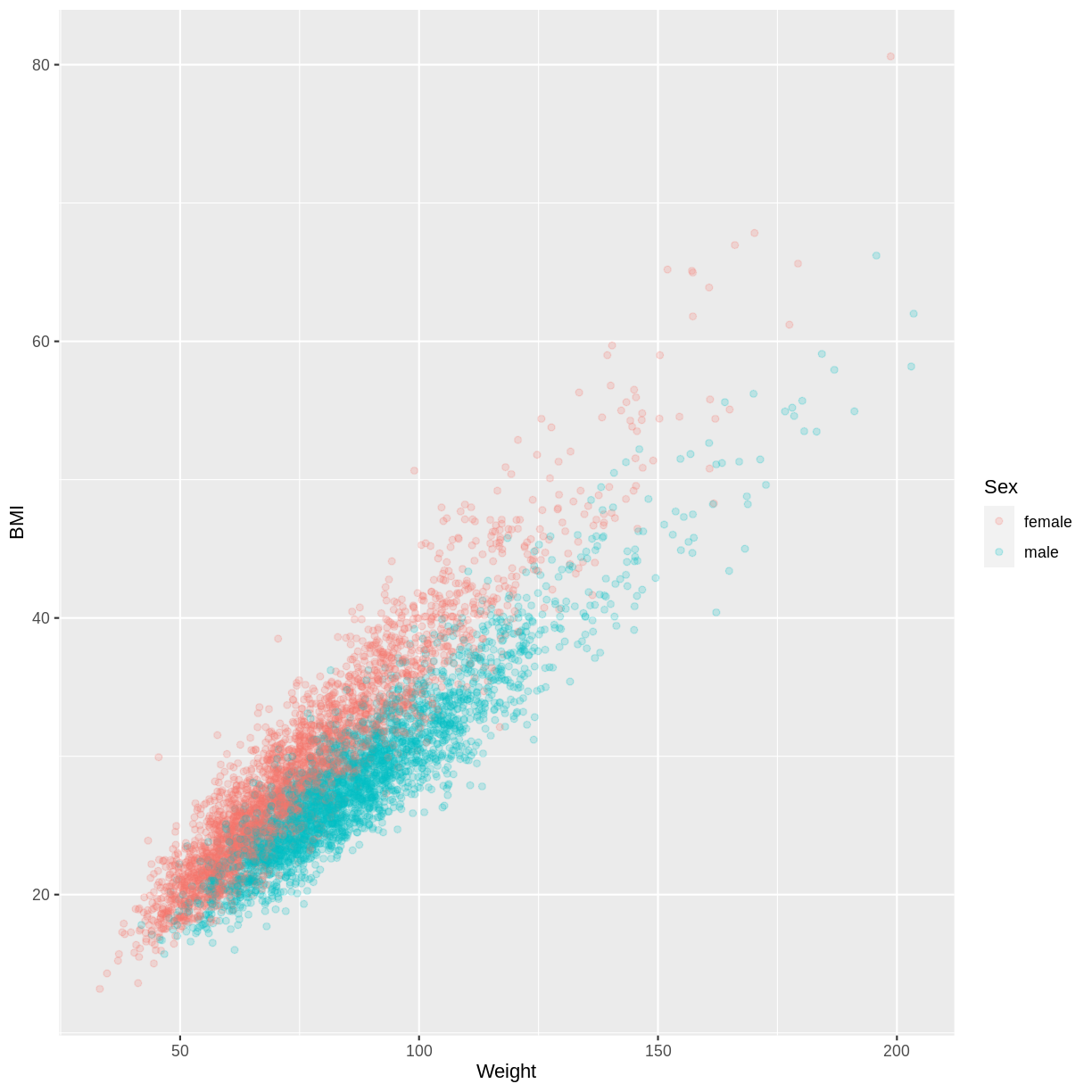
Let us take the response variable BMI, the continuous explanatory variable Weight and the categorical explanatory variable Sex as an example. The code below subsets our data for individuals who are older than 17 years with filter(). The plotting is then initiated using ggplot(). Inside aes(), we select the response variable with y = BMI, the continuous explanatory variable with x = Weight and the categorical explanatory variable with colour = Sex. As a consequence of the final argument, the points produced by geom_point() are coloured by Sex. Finally, we include opacity using alpha = 0.2, which allows us to distinguish areas dense in points from sparser areas. Note that RStudio returns the warning “Removed 320 rows containing missing values (geom_point).” - this reflects that 320 participants had missing BMI and/or Weight data.

The plot suggests that on average, participants classed as female have a higher BMI than participants classed as male, for any particular value of Weight. We might therefore want to account for this in our model by having separate intercepts for the levels of Sex.

dat %>%
  filter(Age > 17) %>%
  ggplot(aes(x = Weight, y = BMI, colour = Sex)) +
  geom_point(alpha = 0.2) 

Exercise

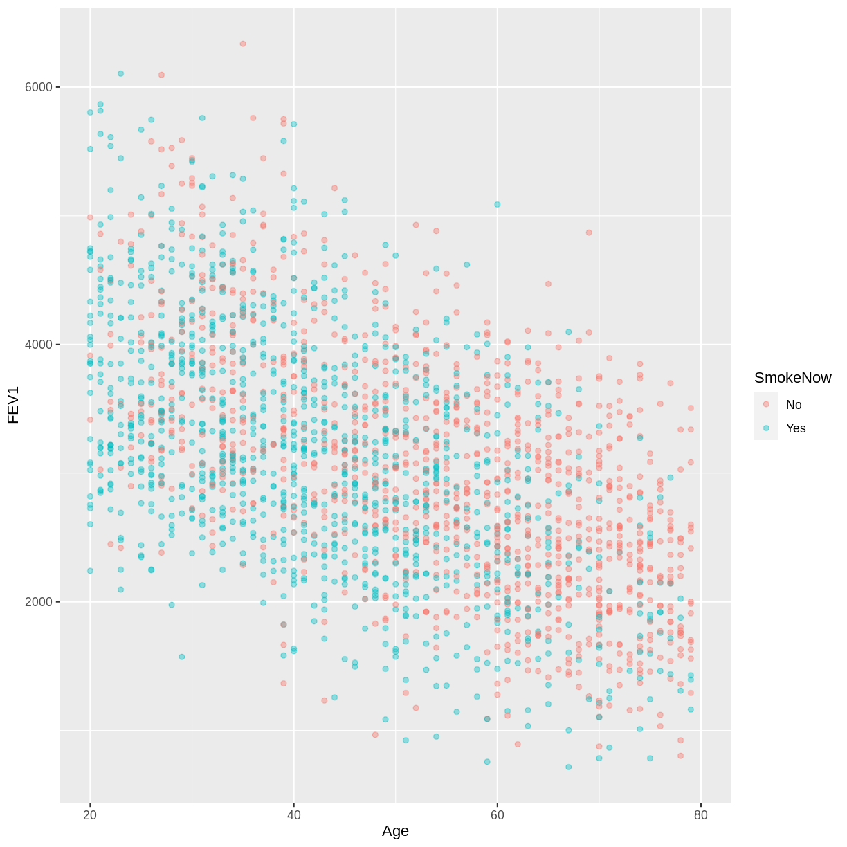
You have been asked to model the relationship between FEV1 and Age in the NHANES data, splitting observations by whether participants are active or ex smokers (SmokeNow). Use the ggplot2 package to create an exploratory plot, ensuring that:

1. NAs are discarded from the SmokeNow variable.
2. FEV1 (FEV1) is on the y-axis and Age (Age) is on the x-axis.
3. These data are shown as a scatterplot, with points coloured by SmokeNow and an opacity of 0.4.

Solution

dat %>%
 drop_na(SmokeNow) %>%
 ggplot(aes(x = Age, y = FEV1, colour = SmokeNow)) +
 geom_point(alpha = 0.4)

Fitting and interpreting a multiple linear regression model

We fit the model using lm(). With formula = BMI ~ Weight + Sex we specify that our model has two explanatory variables, Weight and Sex.

BMI_Weight_Sex <- dat %>%
  filter(Age > 17) %>%
  lm(formula = BMI ~ Weight + Sex)

The linear model equation associated with this model has the general form

[E(y) = \beta_0 + \beta_1 \times x_1 + \beta_2 \times x_2.]

Notice that we now have the additional parameters, $\beta_2$ and $x_2$, in comparison to the simple linear regression model equation. In the context of our model, $\beta_1$ is the parameter for the effect of Weight and $\beta_2$ is the parameter for the effect of Sex. Recall from the simple linear regression lesson that a categorical variable has a baseline level in R. The parameter associated with the categorical variable then estimates the difference in the outcome variable in a group different from the baseline. Since “f” precedes “m” in the alphabet, R takes female as the baseline level. Therefore, $\beta_2$ estimates the difference in BMI between males and females, given a particular value for Weight. $\beta_2$ is only included when $x_2 = 1$, i.e. when the Sex of a participant is male. This results in separate intercepts for the levels of Sex: the intercept for females is given by $\beta_0$ and the intercept for males is given by $\beta_0 + \beta_2$. In this model, the effect of Weight is given by $\beta_1$, irrespective of the Sex of a participant. This results in equal slopes across the levels of Sex.

The model parameters can be obtained using summ() from the jtools package. We include 95% confidence intervals for the parameter estimates using confint = TRUE and three digits after the decimal point using digits = 3. The intercept when Sex = female equals $5.538$ and the intercept when Sex = male equals $5.538 - 4.202 = 1.336$. Notice that in this model, the effect of Weight is $0.310$, regardless of Sex. The model equation can therefore be updated to be:

[E(\text{BMI}) = 5.538 + 0.310 \times \text{Weight} -4.202 \times x_2,]

where $x_2 = 1$ for Sex = male and $0$ otherwise.

summ(BMI_Weight_Sex, confint = TRUE, digits = 3)

MODEL INFO:
Observations: 6177 (320 missing obs. deleted)
Dependent Variable: BMI
Type: OLS linear regression 

MODEL FIT:
F(2,6174) = 19431.981, p = 0.000
R² = 0.863
Adj. R² = 0.863 

Standard errors: OLS
--------------------------------------------------------------
                      Est.     2.5%    97.5%    t val.       p
----------------- -------- -------- -------- --------- -------
(Intercept)          5.538    5.289    5.787    43.656   0.000
Weight               0.310    0.307    0.313   196.965   0.000
Sexmale             -4.202   -4.333   -4.071   -63.075   0.000
--------------------------------------------------------------

Exercise

1. Using the lm() command, fit a multiple linear regression of FEV1 (FEV1) as a function of Age (Age), grouped by SmokeNow. Name this lm object FEV1_Age_SmokeNow.
2. Using the summ function from the jtools package, answer the following questions:

A) What FEV1 does the model predict, on average, for an individual, belonging to the baseline level of SmokeNow, with an Age of 0?
B) What is R taking as the baseline level of SmokeNow and why?
C) By how much is FEV1 expected to differ, on average, between the baseline and the alternative level of SmokeNow?
D) By how much is FEV1 expected to differ, on average, for a one-unit difference in Age?
E) Given these values and the names of the response and explanatory variables, how can the general equation $E(y) = \beta_0 + {\beta}_1 \times x_1 + {\beta}_2 \times x_2$ be adapted to represent the model?

Solution

FEV1_Age_SmokeNow <- dat %>%
  lm(formula = FEV1 ~ Age + SmokeNow)

summ(FEV1_Age_SmokeNow, confint = TRUE, digits=3)

MODEL INFO:
Observations: 2265 (7735 missing obs. deleted)
Dependent Variable: FEV1
Type: OLS linear regression 

MODEL FIT:
F(2,2262) = 560.807, p = 0.000
R² = 0.331
Adj. R² = 0.331 

Standard errors: OLS
--------------------------------------------------------------------
                        Est.       2.5%      97.5%    t val.       p
----------------- ---------- ---------- ---------- --------- -------
(Intercept)         4928.155   4805.493   5050.816    78.787   0.000
Age                  -35.686    -37.799    -33.573   -33.117   0.000
SmokeNowYes         -249.305   -317.045   -181.564    -7.217   0.000
--------------------------------------------------------------------

A) 4928.155 mL
B) No, because “n” precedes “y” in the alphabet.
C) On average, individuals from the two categories are expected to differ by 249.305 mL.
D) It is expected to decrease by 35.686 mL.
E) $E(\text{FEV1}) = 4928.155 - 35.686 \times \text{Age} - 249.305 \times x_2$,
where $x_2 = 1$ for current smokers and $0$ otherwise.

Visualising a multiple linear regression model

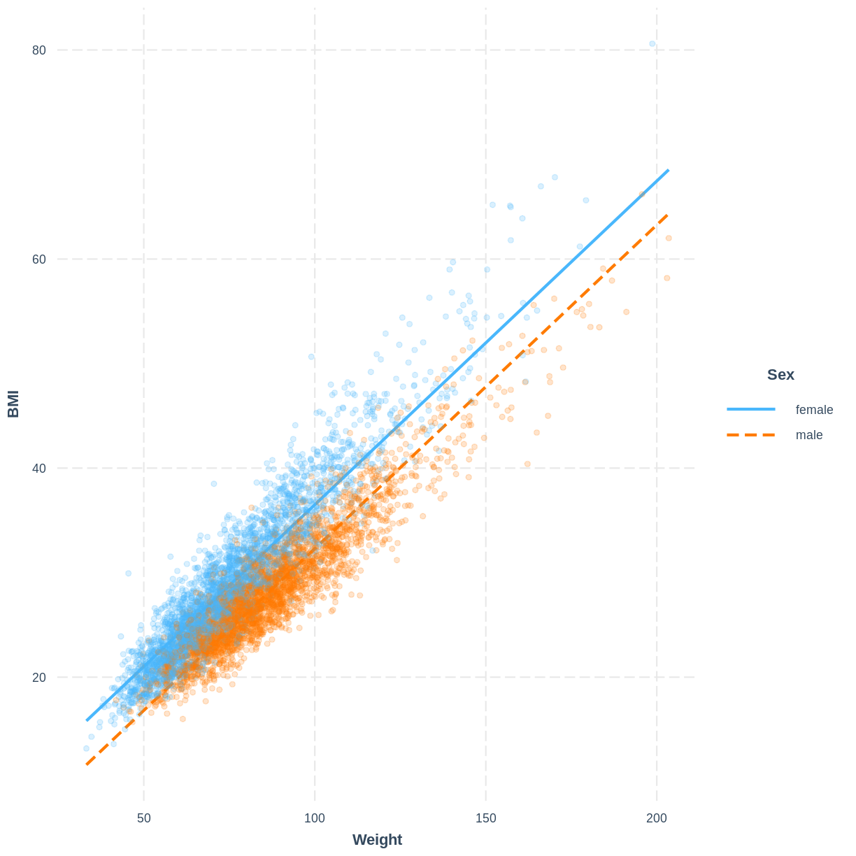
The model can be visualised using two lines, representing the levels of Sex. Rather than using effect_plot() from the jtools package, we use interact_plot from the interactions package. We specify the model by its name, the continuous explanatory variable using pred = Weight and the categorical explanatory variable using modx = Sex. We include the data points using plot.points = TRUE and introduce opacity into the data points using point.alpha = 0.2.

Note that R returns the warning “Weight and Sex are not included in an interaction with one another in the model.” - we will learn what interactions are and when they might be appropriate in the next episode. In this scenario we can safely ignore the warning.

interact_plot(BMI_Weight_Sex, pred = Weight, modx = Sex,
              plot.points = TRUE, point.alpha = 0.2)

Exercise

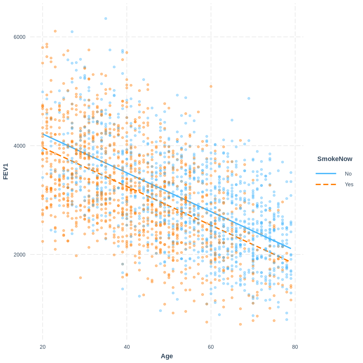
To help others interpret the FEV1_Age_SmokeNow model, produce a figure. Make this figure using the interactions package.

Solution

interact_plot(FEV1_Age_SmokeNow, pred = Age, modx = SmokeNow,
              plot.points = TRUE, point.alpha = 0.4)

Key Points

• A scatterplot, with points coloured by the levels of a categorical variable, can be used to explore the relationship between two continuous variables and a categorical variable.

• The categorical variable can be added to the formula in lm() using a +.

• The model output shows separate intercepts for the levels of the categorical variable. The slope across the levels of the categorical variable is held constant.

• Parallel lines can be added to the exploratory scatterplot to visualise the linear regression model.

Linear regression including an interaction between one continuous and one categorical explanatory variable

Overview

Teaching: 20 min
Exercises: 30 min

Questions

• When is it appropriate to add an interaction to a multiple linear regression model?

• How do we add an interaction term in the lm() command?

• How do the coefficient estimates given by summ() relate to the multiple linear regression model equation?

• How can we visualise the final model in R?

Objectives

• Recognise from an exploratory plot when an interaction between a continuous and a categorical explanatory variable is appropriate.

• Fit a linear regression model including an interaction between one continuous and one categorical explanatory variable using lm().

• Use the jtools package to interpret the model output.

• Use the interactions package to visualise the model output.

In the previous episode, we modeled the effect of the continuous explanatory variable as equal across the groups of the categorical explanatory variable. For example, the effect of Weight on BMI was estimated as $0.31$ for both females and males. In this episode we will expand our modelling approach to include an interaction between the continuous and categorical explanatory variables. As a result, not only the intercept but also the coefficient of the explanatory variable will differ across the levels of the categorical variable in our model. This is appropriate when the slope in our scatterplot differs between the levels of the categorical variable.

Visually exploring the need for an interaction

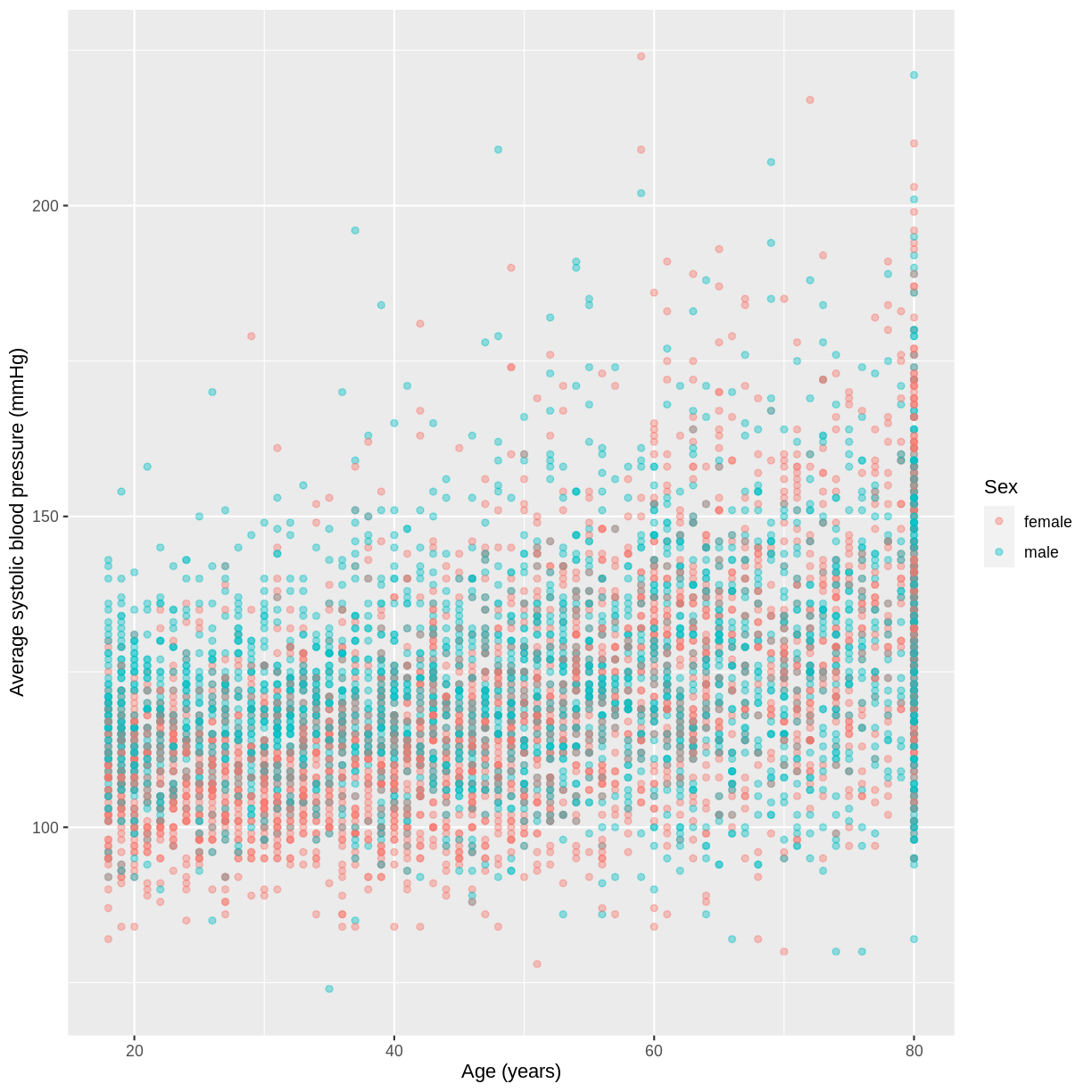
We will use the variables BPSysAve, Age and Sex as an example. Looking at the scatterplot below, for which the data has been filtered to include participants over the age of 17, it seems that the slope for females is greater than for males.

dat %>%
  filter(Age > 17) %>%
  ggplot(aes(x = Age, y = BPSysAve, colour = Sex)) +
  geom_point(alpha = 0.4) +
  ylab("Average systolic blood pressure (mmHg)") +
  xlab("Age (years)")

Exercise

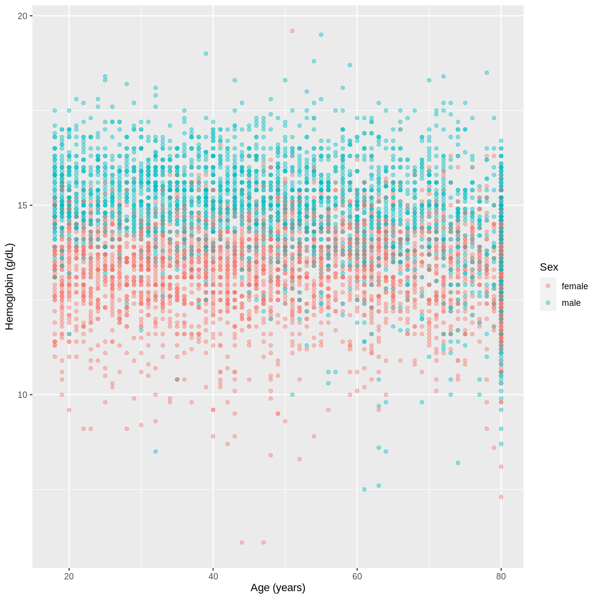
You have been asked to model the relationship between Hemoglobin and Age in the NHANES data, splitting observations by Sex. Use the ggplot2 package to create an exploratory plot, ensuring that:

1. Only participants aged 18 or over are included.
2. Hemoglobin (Hemoglobin) is on the y-axis and Age (Age) is on the x-axis.
3. These data are shown as a scatterplot, with points coloured by Sex and an opacity of 0.4.
4. The axes are labelled as “Hemoglobin (g/dL)” and “Age (years)”.

Solution

dat %>%
  filter(Age > 17) %>%
  ggplot(aes(x = Age, y = Hemoglobin, colour = Sex)) +
  geom_point(alpha = 0.4) +
  ylab("Hemoglobin (g/dL)") +
  xlab("Age (years)")

Fitting and interpreting a multiple linear regression model with an interaction

The code for fitting our model is similar to the previous lm() commands. Notice however that instead of a + between the explanatory variables, we use a *. This is how we tell lm() that we want an interaction between the explanatory variables to be included in the model. The interaction allows the effect of Age to differ across the levels of Sex.

In the output from summ() we see two coefficients that relate to the baseline level of Sex: an intercept and the effect for Age. For the alternative level of Sex, we see two further coefficients: the difference in the intercept (Sexmale) and the difference in the slope (Age:Sexmale). The equation for this model therefore becomes:

\(E(\text{Average systolic blood pressure}) = 93.39 + \left(0.55 \times \text{Age}\right) + \left(17.06 \times x_2\right) - \left(0.28 \times x_2 \times \text{Age}\right)\),

where $x_2 = 1$ for male participants and $0$ otherwise.

Since the difference in the intercepts is positive, we expect a greater intercept for males than for females. Furthermore, since the difference in the slopes is negative, we expect a smaller slope for males than for females.

BPSysAve_Age_Sex <- dat %>%
  filter(Age > 17) %>%
  lm(formula = BPSysAve ~ Age * Sex)

summ(BPSysAve_Age_Sex)

MODEL INFO:
Observations: 5996 (501 missing obs. deleted)
Dependent Variable: BPSysAve
Type: OLS linear regression 

MODEL FIT:
F(3,5992) = 552.67, p = 0.00
R² = 0.22
Adj. R² = 0.22 

Standard errors: OLS
------------------------------------------------
                     Est.   S.E.   t val.      p
----------------- ------- ------ -------- ------
(Intercept)         93.39   0.80   116.27   0.00
Age                  0.55   0.02    35.63   0.00
Sexmale             17.06   1.15    14.89   0.00
Age:Sexmale         -0.28   0.02   -12.68   0.00
------------------------------------------------

Exercise

1. Using the lm() command, fit a multiple linear regression model of Hemoglobin (Hemoglobin) as a function of Age (Age), grouped by Sex, including an interaction between Age and Sex. Make sure to only include participants who were 18 years or older. Name the lm object Hemoglobin_Age_Sex.
2. Using the summ function from the jtools package, answer the following questions:

A) What concentration of Hemoglobin does the model predict, on average, for an individual, belonging to the baseline level of Sex, with an Age of 0?
B) By how much is Hemoglobin expected to differ, on average, for the alternative level of Sex, at an Age of 0?
C) By how much is Hemoglobin expected to differ, on average, for a one-unit difference in Age in the baseline level of Sex?
D) By how much is Hemoglobin expected to differ, on average, for a one-unit difference in Age in the alternative level of Sex?
E) Given these values and the names of the response and explanatory variables, how can the general equation $E(y) = \beta_0 + {\beta}_1 \times x_1 + {\beta}_2 \times x_2 + {\beta}_3 \times x_1 \times x_2$ be adapted to represent the model?

Solution

Hemoglobin_Age_Sex <- dat %>%
  filter(Age > 17) %>%
  lm(formula = Hemoglobin ~ Age * Sex)

summ(Hemoglobin_Age_Sex)

MODEL INFO:
Observations: 5995 (502 missing obs. deleted)
Dependent Variable: Hemoglobin
Type: OLS linear regression 

MODEL FIT:
F(3,5991) = 1026.31, p = 0.00
R² = 0.34
Adj. R² = 0.34 

Standard errors: OLS
------------------------------------------------
                     Est.   S.E.   t val.      p
----------------- ------- ------ -------- ------
(Intercept)         13.29   0.06   219.70   0.00
Age                  0.00   0.00     0.68   0.49
Sexmale              2.76   0.09    31.85   0.00
Age:Sexmale         -0.02   0.00   -13.94   0.00
------------------------------------------------

A) 13.29 g/dL.
B) On average, individuals from the two categories are expected to differ by 2.76 g/dL at an Age of 0.
C) On average, female participants with a one-unit difference in Age are expected to differ by 0.00 in their Hemoglobin concentration. So, not at all.
D) On average, male participants with a one-unit difference in Age are expected to differ by 0.02 in their Hemoglobin concentration.
E) $E(\text{Hemoglobin}) = 13.29 + 0.00 \times \text{Age} + 2.76 \times x_2 - 0.02 \times \text{Age} \times x_2$, where $x_2 = 1$ for participants of the male Sex and $0$ otherwise.

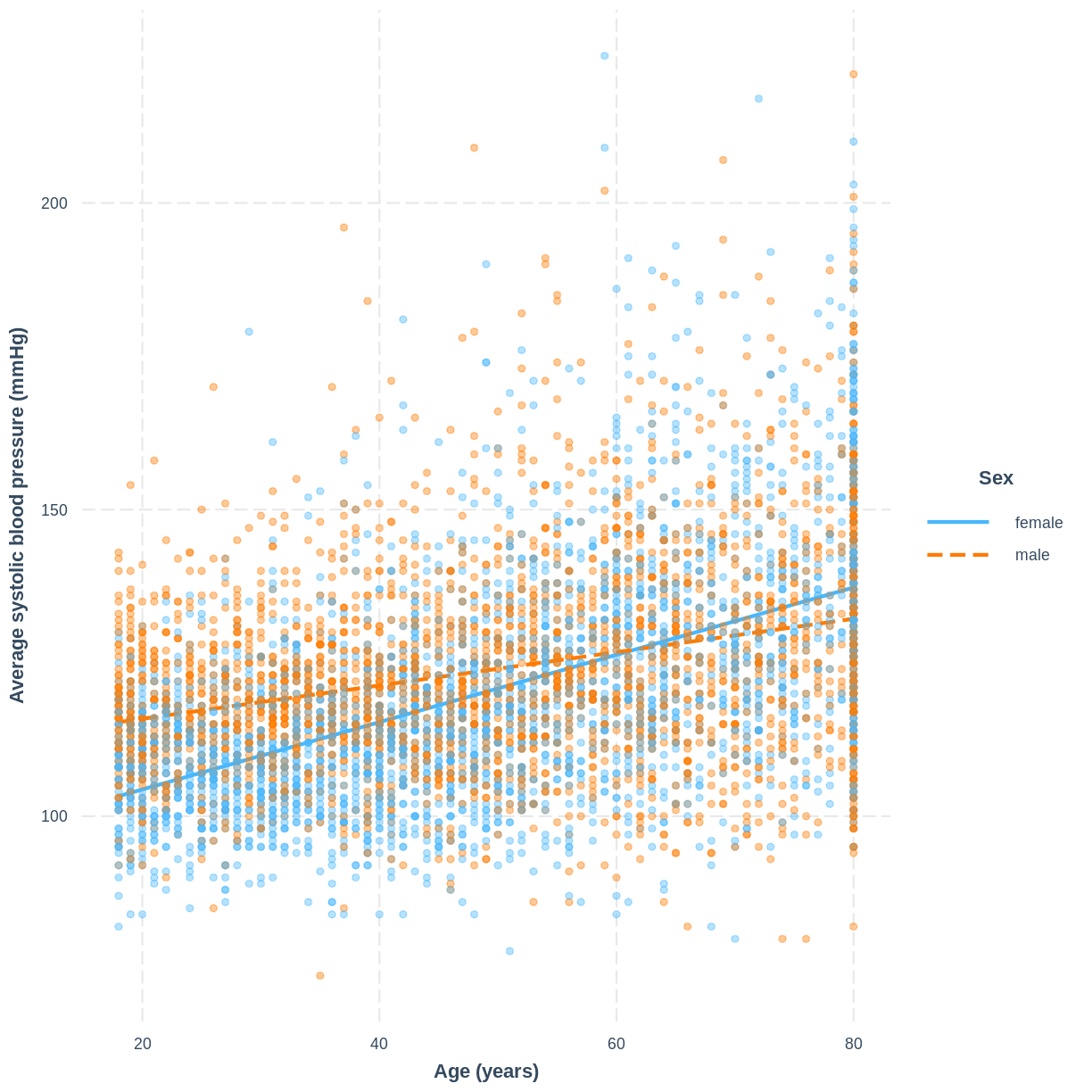
Visualising a multiple linear regression model with an interaction

We can visualise the model, as before, using the interact_plot() function.

interact_plot(BPSysAve_Age_Sex, pred = Age, modx = Sex,
              plot.points = TRUE, point.alpha = 0.4) +
  ylab("Average systolic blood pressure (mmHg)") +
  xlab("Age (years)")

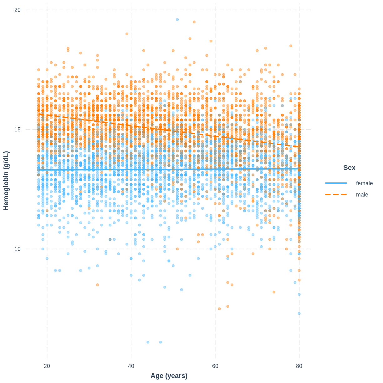
Exercise

To help others interpret the Hemoglobin_Age_Sex model, produce a figure. Make this figure using the interactions package.

Solution

interact_plot(Hemoglobin_Age_Sex, pred = Age, modx = Sex, 
              plot.points = TRUE, point.alpha = 0.4) +
  ylab("Hemoglobin (g/dL)") +
  xlab("Age (years)")

Key Points

• It may be appropriate to include an interaction when the slopes appear to differ across levels of a categorical variable.

• Replace + by * in the lm() command to add an interaction.

• When an interaction is included, two coefficients relate to differences between the two levels of a categorical variable - one relates to a difference in the intercept, the other to a difference in the slope.

• The function interact_plot() can be used to visualise the model.

Making predictions from a multiple linear regression model

Overview

Teaching: 8 min
Exercises: 12 min

Questions

• How can we make predictions using the model equation of a multiple linear regression model?

• How can we use R to obtain predictions from a multiple linear regression model?

Objectives

• Calculate a prediction from a simple linear regression model using parameter estimates given by the model output.

• Use the predict function to generate predictions from a multiple linear regression model.

As with the simple linear regression model, the multiple linear regression model allows us to make predictions. First we will calculate predictions using the model equation. Then we will see how R can calculate predictions for us using the make_predictions() function.

Calculating predictions manually

Let us use the BPSysAve_Age_Sex model from the previous episode. The equation for this model was:

\(E(\text{BPSysAve}) = 93.39 + 0.55 \times \text{Age} + 17.06 \times x_2 - 0.28 \times x_2 \times \text{Age}\),

where $x_2 = 1$ for male participants and $0$ otherwise.

For a 30-year old female, the model predicts an average systolic blood pressure of

\(E(\text{BPSysAve}) = 93.39 + 0.55 \times 30 + 17.06 \times 0 - 0.28 \times 0 \times 30 = 93.39 + 16.5 = 109.89\).

For a 30-year old male, the model predicts an average systolic blood pressure of

\(E(\text{BPSysAve}) = 93.39 + 0.55 \times 30 + 17.06 \times 1 - 0.28 \times 1 \times 30 = 93.39 + 16.5 + 17.06 - 8.4 = 118.55\).

Exercise

Given the summ output from our Hemoglobin_Age_Sex model, the model can be described as \(E(\text{Hemoglobin}) = 13.29 + 0.00 \times \text{Age} + 2.76 \times x_2 - 0.02 \times x_2 \times \text{Age}\), where $x_2 = 1$ for participants of the male Sex and $0$ otherwise.

1. What level of Hemoglobin does the model predict, on average, for an individual of the female Sex with an Age of 40?
2. What Hemoglobin is predicted for a male of the same Age?

Solution

For 40-year old females: $13.29 + 0.00 \times 40 + 2.76 \times 0 - 0.02 \times 0 \times 40 = 13.29$.
For 40-year old males: $13.29 + 0.00 \times 40 + 2.76 \times 1 - 0.02 \times 1 \times 40 = 13.29 + 2.76 - 0.8 = 15.25$.

Making predictions using make_predictions()

Using the make_predictions() function brings two advantages. First, when calculating multiple predictions, we are saved the effort of inserting multiple values into our model manually and doing the calculations. Secondly, make_predictions() returns 95% confidence intervals around the predictions, giving us a sense of the uncertainty around the predictions.

To use make_predictions(), we need to create a tibble with the explanatory variable values for which we wish to have mean predictions from the model. We do this using the tibble() function. Note that the column names must correspond to the names of the explanatory variables in the model, i.e. Age and Sex. In the code below, we create a tibble with Age having the values 30, 40, 50 and 60 for females and males. We then provide make_predictions() with this tibble, alongside the model from which we wish to have predictions. By default, make_predicitons() returns 95% confidence intervals for the mean predictions.

From the output we can see that the model predicts an average systolic blood pressure of 109.8596 for a 30-year old female. The confidence interval around this prediction is [109.0593, 110.6599].

BPSysAve_Age_Sex <- dat %>%
  filter(Age > 17) %>%
  lm(formula = BPSysAve ~ Age * Sex)

predictionDat <- tibble(Age = c(30, 40, 50, 60,
                                30, 40, 50, 60),
                        Sex = c("female", "female", "female", "female",
                                "male", "male", "male", "male"))

make_predictions(BPSysAve_Age_Sex, new_data = predictionDat)

# A tibble: 8 × 5
    Age Sex    BPSysAve  ymin  ymax
  <dbl> <chr>     <dbl> <dbl> <dbl>
1    30 female     110.  109.  111.
2    40 female     115.  115.  116.
3    50 female     121.  120.  121.
4    60 female     126.  126.  127.
5    30 male       119.  118.  119.
6    40 male       121.  121.  122.
7    50 male       124.  123.  125.
8    60 male       127.  126.  127.

Exercise

Using the make_predictions() function, obtain the expected mean Hemoglobin levels predicted by the Hemoglobin_Age_Sex model for individuals with an Age of 20, 30, 40 and 50. Obtain confidence intervals for these predictions. How are these confidence intervals interpreted?

Solution

Hemoglobin_Age_Sex <- dat %>%
 filter(Age > 17) %>%
 lm(formula = Hemoglobin ~ Age * Sex)

predictionDat <- tibble(Age = c(20, 30, 40, 50,
                                 20, 30, 40, 50),
                         Sex = c("female", "female", "female", "female",
                                 "male", "male", "male", "male"))

make_predictions(Hemoglobin_Age_Sex, new_data = predictionDat)

# A tibble: 8 × 5
    Age Sex    Hemoglobin  ymin  ymax
  <dbl> <chr>       <dbl> <dbl> <dbl>
1    20 female       13.3  13.2  13.4
2    30 female       13.3  13.3  13.4
3    40 female       13.3  13.3  13.4
4    50 female       13.3  13.3  13.4
5    20 male         15.6  15.5  15.7
6    30 male         15.4  15.3  15.4
7    40 male         15.2  15.1  15.2
8    50 male         14.9  14.9  15.0

Recall that 95% of the 95% confidence intervals are expected to contain the population mean. Therefore, we can be fairly confident that the true population means lie somewhere between the bounds of the intervals, assuming that our model is good.

Key Points

• Predictions of the mean in the outcome variable can be manually calculated using the model’s equation.

• Predictions of multiple means in the outcome variable alongside 95% CIs can be obtained using the make_predictions() function.

Assessing multiple linear regression model fit and assumptions

Overview

Teaching: 15 min
Exercises: 45 min

Questions

• Why is the adjusted R squared used, instead of the standard R squared, when working with multiple linear regression?

• What are the six assumptions of multiple linear regression and how are they assessed?

Objectives

• Use the adjusted R squared value as a measure of model fit.

• Assess whether the assumptions of the multiple linear regression model have been violated.

In this episode we will check the fit and assumptions of multiple linear regression models. We will use the extension to $R^2$ for multiple linear regression models, the adjusted $R^2$ ($R^2_{adj}$). We will also learn to assess the six linear regression assumptions in the case of multiple linear regression.

Measuring fit using $R^2_{adj}$

In the simple linear regression episode on model assumptions we learned that $R^2$ quantifies the proportion of variation in the outcome variable explained by the explanatory variable. In the context of multiple linear regression, a caveat emerges to $R^2$: adding explanatory variables to our model will always increase $R^2$, even if the explanatory variables are not related to the response variable. Therefore, when interpreting the output from summ(), look at the $R^2_{adj}$. This is an $R^2$ corrected for the number of variables in the model. In some cases, the adjusted and unadjusted metrics will be (near) equal. In other cases, the differences will be larger.

Exercise

Find the adjusted R-squared value for the summ output of our Hemoglobin_Age_Sex model from episode 2. What proportion of variation in hemoglobin is explained by age, sex and their interaction in our model? Does our model account for most of the variation in Hemoglobin?

Solution

Hemoglobin_Age_Sex <- dat %>%
  filter(Age > 17) %>%
  lm(formula = Hemoglobin ~ Age * Sex)

summ(Hemoglobin_Age_Sex, confint = TRUE)

MODEL INFO:
Observations: 5995 (502 missing obs. deleted)
Dependent Variable: Hemoglobin
Type: OLS linear regression 

MODEL FIT:
F(3,5991) = 1026.31, p = 0.00
R² = 0.34
Adj. R² = 0.34 

Standard errors: OLS
---------------------------------------------------------
                     Est.    2.5%   97.5%   t val.      p
----------------- ------- ------- ------- -------- ------
(Intercept)         13.29   13.18   13.41   219.70   0.00
Age                  0.00   -0.00    0.00     0.68   0.49
Sexmale              2.76    2.59    2.93    31.85   0.00
Age:Sexmale         -0.02   -0.03   -0.02   -13.94   0.00
---------------------------------------------------------

Since $R^2_{adj} = 0.34$, our model accounts for approximately 34% of the variation in Hemoglobin. Our model explains 34% of the variation in Hemoglobin, which a model that always predicts the mean would not.

Assessing the assumptions of the multiple linear regression model

We learned to assess six assumptions in the simple linear regression episode on model assumptions. These assumptions also hold in the multiple linear regression context, although in some cases their assessment is a little more extensive. Below we will practice assessing these assumptions.

Validity

Recall that the validity assumption states that the model is appropriate for the research question. Validity is assessed through three questions:

A) Does the outcome variable reflect the phenomenon of interest?
B) Does the model include all relevant explanatory variables?
C) Does the model generalise to our case of interest?

Exercise

You are asked to use the FEV1_Age_SmokeNow model to answer the following research question:

“Does the effect of age on FEV1 differ by smoking status in US adults?”

Using the three points above, assess the validity of this model for the research question.

Solution

A) The research question is on FEV1, which is our outcome variable. Therefore our outcome variable reflects the phenomenon of interest.
B) Our research question asks whether the effect of age differs by smoking status, which can be tested using an interaction between Age and SmokeNow. Since our model does not include this interaction, our model does not include all relevant explanatory variables.
C) Since the NHANES data was collected from individuals in the US, our model should generalise to our case of interest.

Representativeness

Recall that the representativeness assumption states that the sample is representative of the population to which we are generalising our findings. This assumption is assessed in the same way as for the case of the simple linear regression model, so we will not go through another exercise at this point. Note however that when representativesness is violated, this can sometimes be solved by adding the misrepresented variable to the model as an extra explanatory variable.

Linearity and additivity

Recall that this assumption states that our outcome variable has a linear, additive relationship with the explanatory variables.

The linearity component is assessed in the same way as in the simple linear regression case. For example, recall that the relationship between combined diastolic blood pressure (BPDiaAve) and age in months (AgeMonths) was curved (see this episode from the simple linear regression lesson). Adding a squared term to the model helped us to model this non-linear relationship. We can add a Sex term to fit separate non-linear curves to this data:

BPDiaAve_AgeMonthsSQ_Sex <- lm(BPDiaAve ~ AgeMonths + I(AgeMonths^2) + Sex, data = dat)
interact_plot(BPDiaAve_AgeMonthsSQ_Sex, pred = AgeMonths, modx = Sex,
            plot.points = TRUE, interval = TRUE,
            point.size = 0.7) +
  ylab("Combined diastolic blood pressure") +
  xlab("Age in Months") 

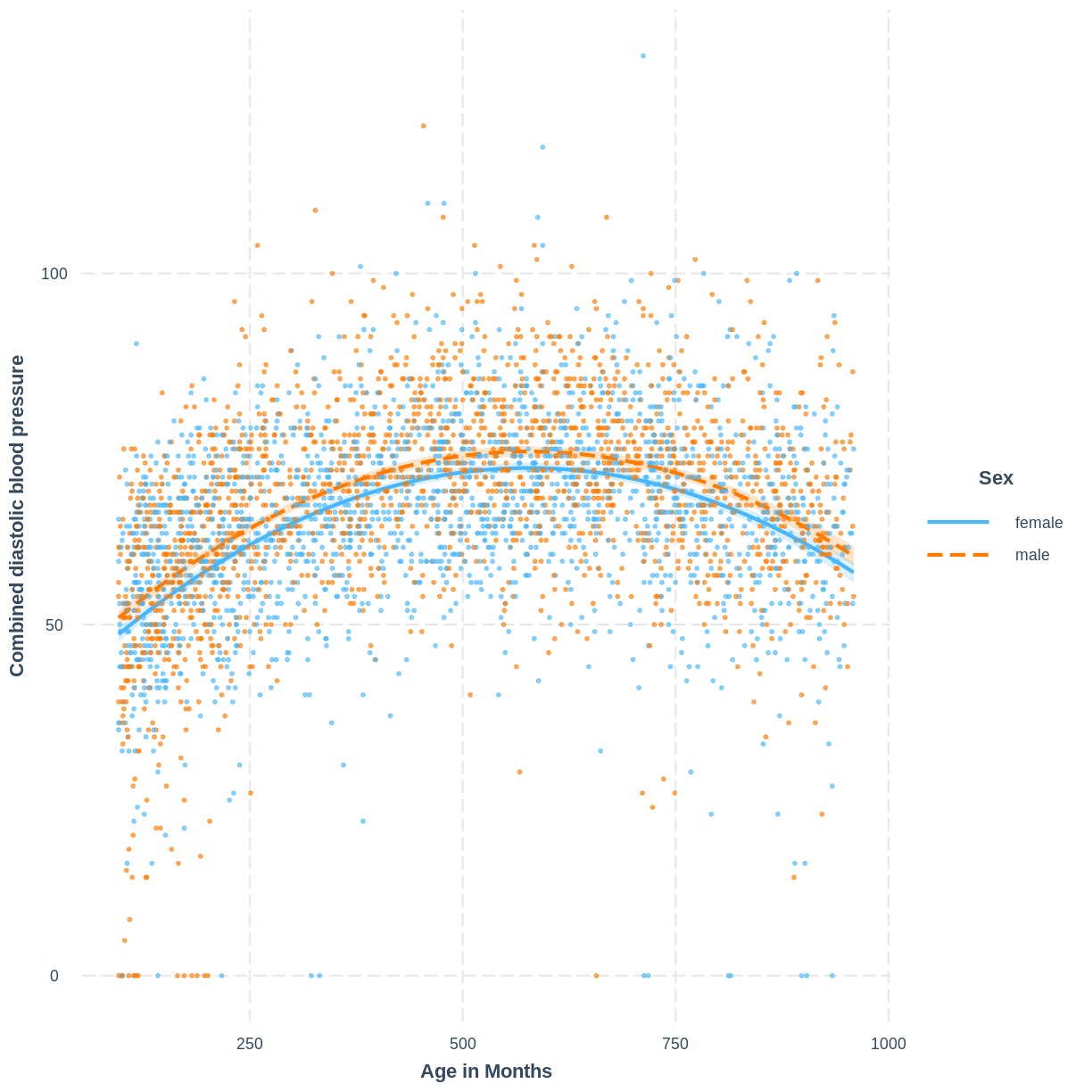
The non-linear relationship has now been modeled separately for levels of a categorical variable.

Recall that the additivity component of the linearity and additivity assumption means that the effect of any explanatory variable on the outcome variable does not depend on another explanatory variable in the model. In other words, that our model includes all necessary interactions between explanatory variables. In the above example, the additivity component does not appear to be violated: it does not look like the data requires an interaction between age and sex. However, to be sure of this we may compare the model fit of models with and without the interaction using the tools discussed in this episode.

Exercise

In the example above we saw that a model with a squared explanatory variable can also include separate intercepts for levels of a categorical variable.

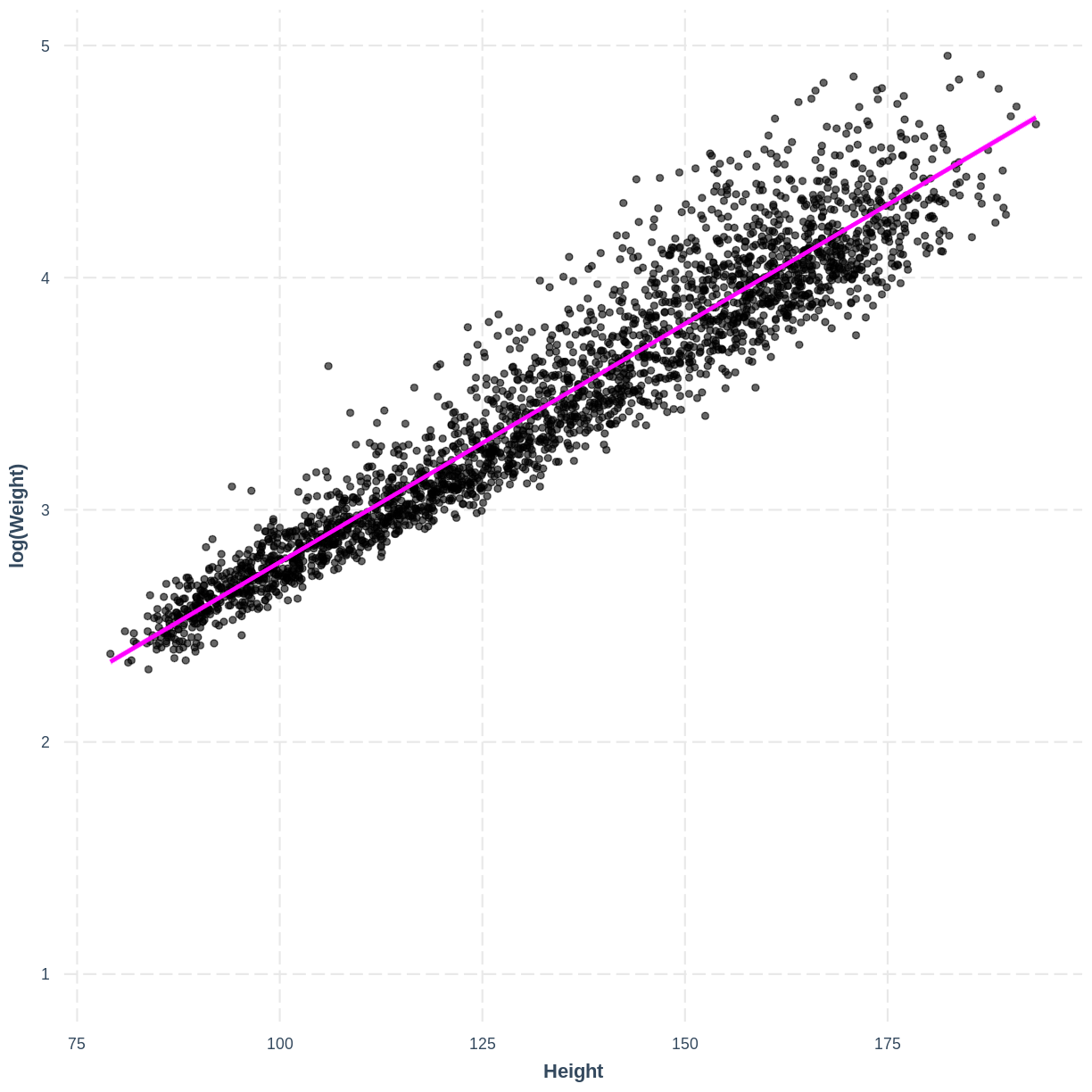
Recall our child_logWeight_Height_lm model from the previous lesson, which modeled the relationship between the log of child weight and child height:

child_logWeight_Height_lm <- dat %>%
  filter(Age < 18) %>%
  lm(formula = log(Weight) ~ Height)

effect_plot(child_logWeight_Height_lm, pred = Height, 
                  plot.points = TRUE, interval = TRUE,
                  line.colors = c("magenta")) 

Extend this model by adding separate intercepts for the levels of the Sex variable. Visualise the model using interact_plot(). Do you think that including the interaction between Height and Sex is necessary?

Solution

child_logWeight_Height_Sex <- dat %>%
  filter(Age < 18) %>%
  lm(formula = log(Weight) ~ Height + Sex)

interact_plot(child_logWeight_Height_Sex, pred = Height, modx = Sex,
              plot.points = TRUE, interval = TRUE,
              point.size = 0.7)

There is little evidence from the plot that the effect of height on weight is different between sexes meaning that an interaction term is not needed. But we could assess the model fit with and without the interaction to check.

Independent errors

Recall that when observations in our data are grouped, this can result in a violation of the independent errors assumption. If there are a few levels in our grouping variable (say, less than 6) then we may overcome the violation by including the grouping variable as an explanatory variable in our model. If the grouping variable has many more levels, we may opt for a modelling approach more complex than multiple linear regression.

Exercise

In which of the following scenarios are we at risk of violating the independent errors assumption? In those cases, should we be working with an extra explanatory variable?

A) We are modelling the effect of average daily calorie intake on BMI in the adult UK population. We have one observation per participant and participants are known to belong to one of five income brackets.
B) We are modelling the effect of age on grip strength in adult females in the UK. Whether participants are physically active is known.
C) We are asking whether people’s sprinting speed is increased after partaking in an athletics course. Our data includes measurements of 100 participant’s sprinting speed before and after the course.

Solution

A) Since we have multiple observations per income bracket, our observations are not independent. There are five levels in the income bracket variable, so we may chose to include income bracket as an explanatory variable.
B) Since we have multiple observations per level of physical activity, our observations are not independent. Since there are two levels in our physical activity variable, we could use physical activity as an explanatory variable in our model.
C) This data has two levels of grouping: within individuals (two measurements per individual) and timing (before/after the course). While timing can be included as an explanatory variable (two levels), it would not be appropriate to include individuals as an explanatory variable (100 levels). In this scenario we would opt for a more complex modelling approach (a mixed effect model).

Equal variance of errors (homoscedasticity)

This assumption states that the magnitude of variation in the residuals is not different across the fitted values or any explanatory variable. Importantly, when interactions are included in the model, the scale of the residuals should be checked at the interaction level. In the case of an interaction between continuous and categorical explanatory variables, this means colouring the points in the residuals vs explanatory variable plot by the levels of a categorical variable.

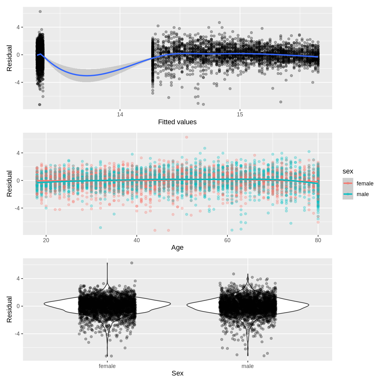
For example, below we create the diagnostic plots for our Hemoglobin_Age_Sex model. We create plots of residuals vs. fitted (p1), residuals vs. age (p2) and residuals vs. sex (p3). Notice that in the residuals vs. age plot, we colour points by sex using colour = sex. This allows us to assess whether the residuals are homogenously scattered across age, grouped by sex (i.e. at the interaction level). Note that the / in p1 / p2 / p3 relies on the patchwork package being loaded and results in the three graphs being plotted in vertical sequence.

residualData <- tibble(resid = resid(Hemoglobin_Age_Sex),
                       fitted = fitted(Hemoglobin_Age_Sex),
                       age = Hemoglobin_Age_Sex$model$Age,
                       sex = Hemoglobin_Age_Sex$model$Sex)

p1 <- ggplot(residualData, aes(x = fitted, y = resid)) +
  geom_point(alpha = 0.3) +
  geom_smooth() +
  ylab("Residual") +
  xlab("Fitted values")

p2 <- ggplot(residualData, aes(x = age, y = resid, colour = sex)) +
  geom_point(alpha = 0.3) +
  geom_smooth() +
  ylab("Residual") +
  xlab("Age")

p3 <- ggplot(residualData, aes(x = sex, y = resid)) +
  geom_violin() + 
  geom_jitter(alpha = 0.3, width = 0.2) +
  ylab("Residual") +
  xlab("Sex")


p1 / p2 / p3

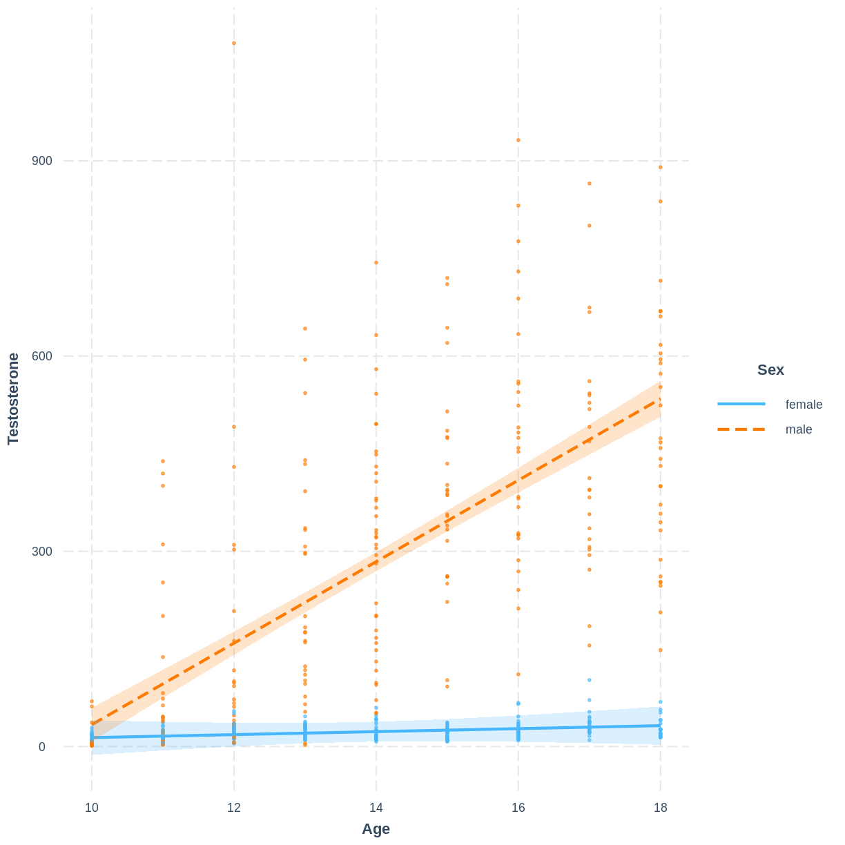
Exercise

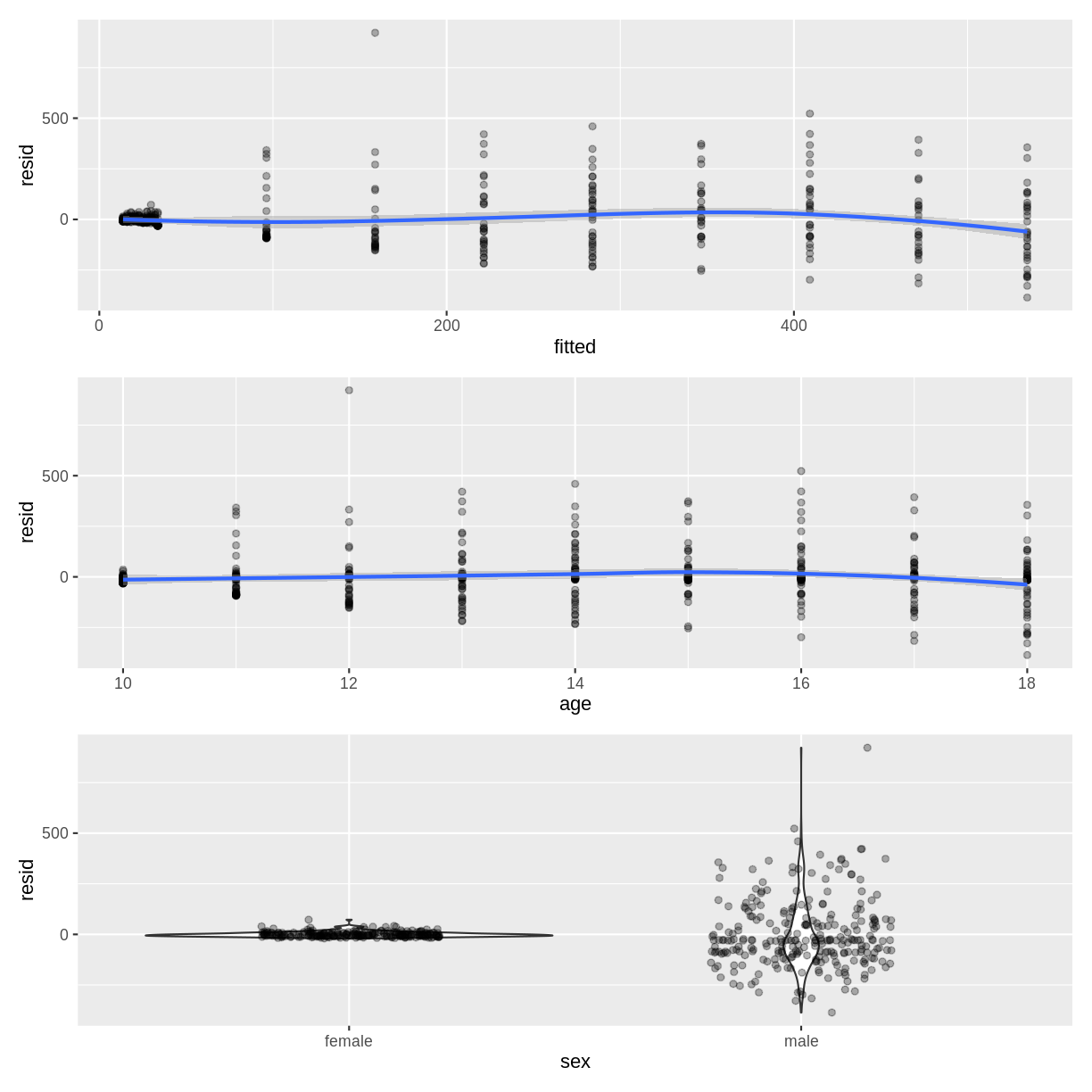
A colleague is studying testosterone levels in children. They have fit a multiple linear regression model of testosterone as a function of age, sex and their interaction. The data and their model look as shown below:

This colleague approaches you for your thoughts on the following diagnostic plots, used to assess the homoscedasticity assumption.

A) What issues can you identify in the diagnostic plots?
B) How could the diagnostic plots be improved to be more informative?

Solution

A) The residuals appear to fan out as the fitted values or age increase. The residuals also do not appear to be homogenous across sex, as the violin plot for males is much longer than for females.
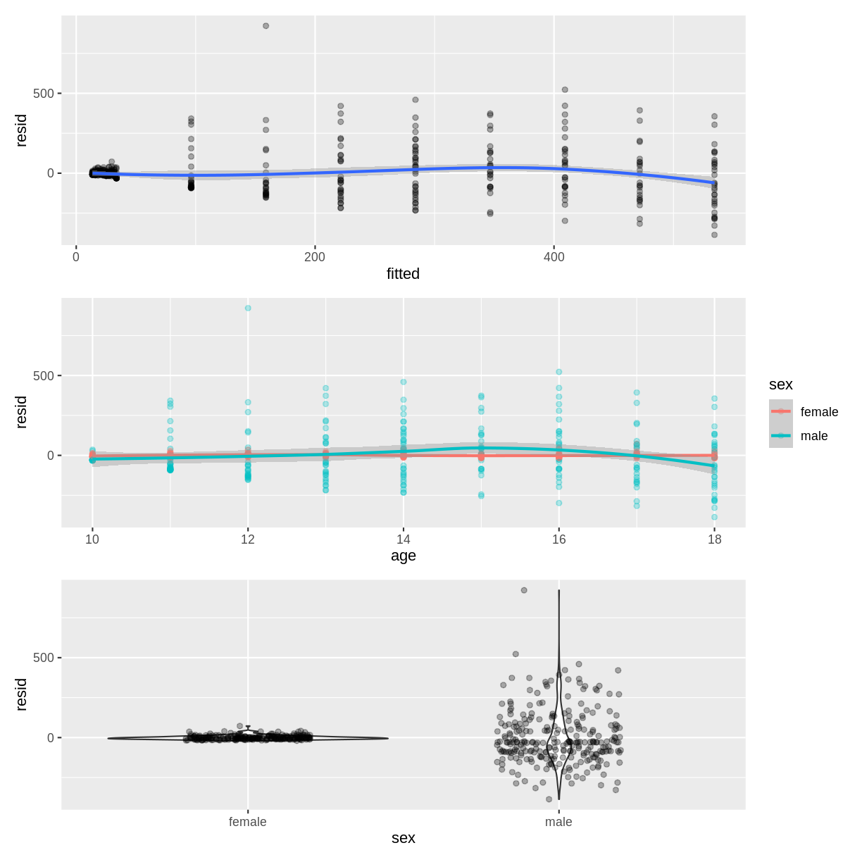
B) The points in the scatterplot of age could be coloured by sex to assess the homoscedasticity assumption at the interaction level:

Normality of errors

Recall that this assumption states that the errors follow a normal distribution. When this assumption is strongly violated, predictions from the model are less reliable. Small deviations from normality may pose less of an issue. This assumption is assessed in the same way as for the case of the simple linear regression model, so we will not go through another exercise at this point.

Key Points

• The adjusted R squared measure ensures that the metric does not increase simply due to the addition of a variable. The variable needs to improve model fit for the adjusted R squared to increase.

• The same assumptions hold for simple and multiple linear regression, however more steps are involved in the assessment of the assumptions in the context of multiple linear regression.