Linear regression including an interaction between one continuous and one categorical explanatory variable
Overview
Teaching: 20 min
Exercises: 30 minQuestions
When is it appropriate to add an interaction to a multiple linear regression model?
How do we add an interaction term in the
lm()command?How do the coefficient estimates given by
summ()relate to the multiple linear regression model equation?How can we visualise the final model in R?
Objectives
Recognise from an exploratory plot when an interaction between a continuous and a categorical explanatory variable is appropriate.
Fit a linear regression model including an interaction between one continuous and one categorical explanatory variable using
lm().Use the jtools package to interpret the model output.
Use the interactions package to visualise the model output.
In the previous episode, we modeled the effect of the continuous explanatory variable as equal across the groups of the categorical explanatory variable. For example, the effect of Weight on BMI was estimated as $0.31$ for both females and males. In this episode we will expand our modelling approach to include an interaction between the continuous and categorical explanatory variables. As a result, not only the intercept but also the coefficient of the explanatory variable will differ across the levels of the categorical variable in our model. This is appropriate when the slope in our scatterplot differs between the levels of the categorical variable.
Visually exploring the need for an interaction
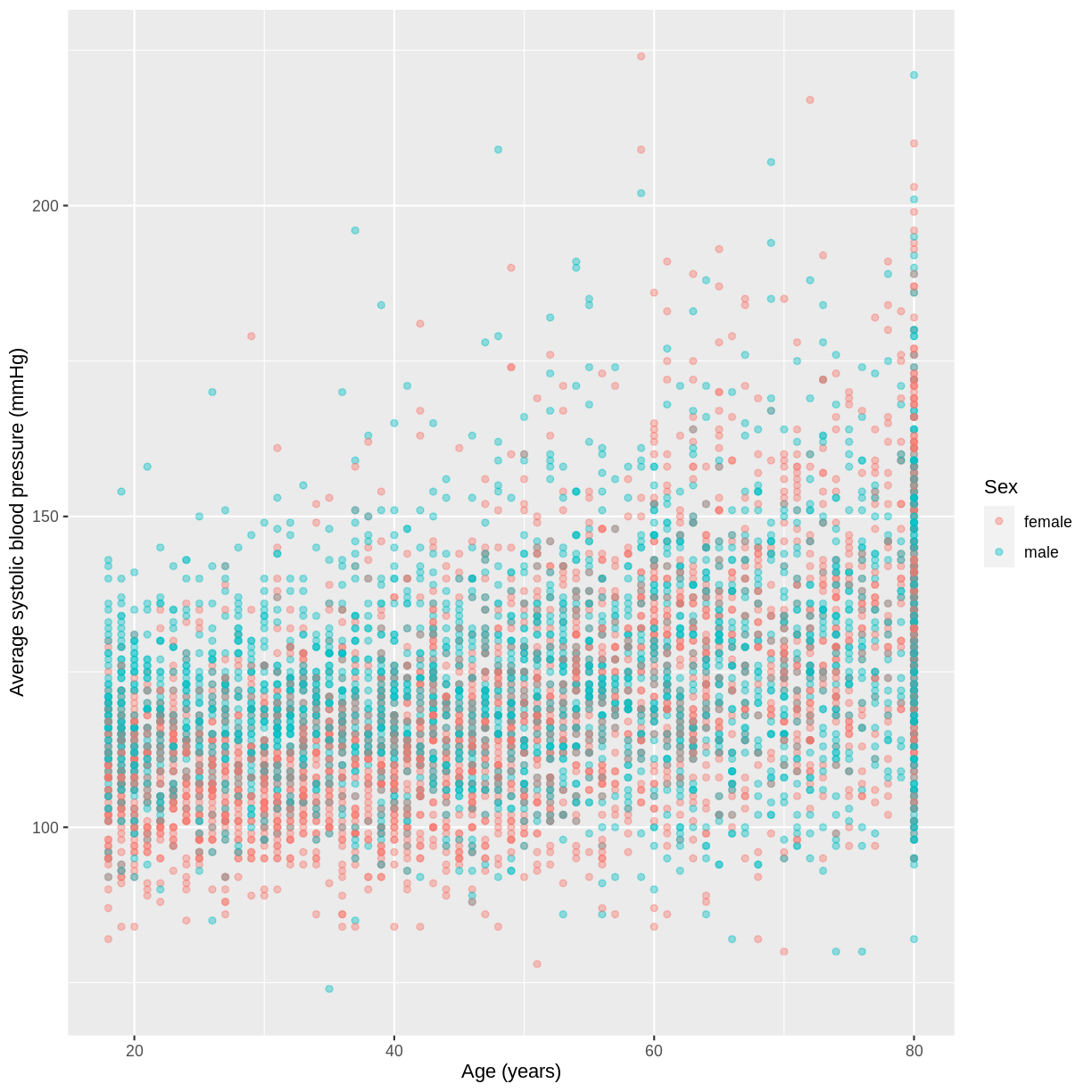
We will use the variables BPSysAve, Age and Sex as an example. Looking at the scatterplot below, for which the data has been filtered to include participants over the age of 17, it seems that the slope for females is greater than for males.
dat %>%
  filter(Age > 17) %>%
  ggplot(aes(x = Age, y = BPSysAve, colour = Sex)) +
  geom_point(alpha = 0.4) +
  ylab("Average systolic blood pressure (mmHg)") +
  xlab("Age (years)")
Exercise
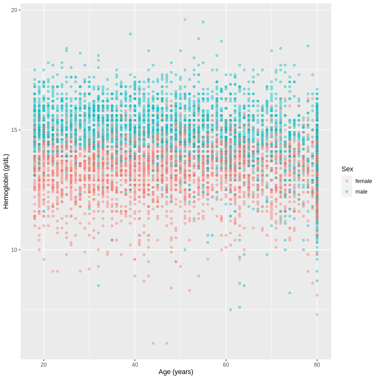
You have been asked to model the relationship between
HemoglobinandAgein the NHANES data, splitting observations bySex. Use theggplot2package to create an exploratory plot, ensuring that:
- Only participants aged 18 or over are included.
- Hemoglobin (
Hemoglobin) is on the y-axis and Age (Age) is on the x-axis.- These data are shown as a scatterplot, with points coloured by
Sexand an opacity of 0.4.- The axes are labelled as “Hemoglobin (g/dL)” and “Age (years)”.
Solution
dat %>%
  filter(Age > 17) %>%
  ggplot(aes(x = Age, y = Hemoglobin, colour = Sex)) +
  geom_point(alpha = 0.4) +
  ylab("Hemoglobin (g/dL)") +
  xlab("Age (years)")
Fitting and interpreting a multiple linear regression model with an interaction
The code for fitting our model is similar to the previous lm() commands. Notice however that instead of a + between the explanatory variables, we use a *. This is how we tell lm() that we want an interaction between the explanatory variables to be included in the model. The interaction allows the effect of Age to differ across the levels of Sex.
In the output from summ() we see two coefficients that relate to the baseline level of Sex: an intercept and the effect for Age. For the alternative level of Sex, we see two further coefficients: the difference in the intercept (Sexmale) and the difference in the slope (Age:Sexmale). The equation for this model therefore becomes:
\(E(\text{Average systolic blood pressure}) = 93.39 + \left(0.55 \times \text{Age}\right) + \left(17.06 \times x_2\right) - \left(0.28 \times x_2 \times \text{Age}\right)\),
where $x_2 = 1$ for male participants and $0$ otherwise.
Since the difference in the intercepts is positive, we expect a greater intercept for males than for females. Furthermore, since the difference in the slopes is negative, we expect a smaller slope for males than for females.
BPSysAve_Age_Sex <- dat %>%
  filter(Age > 17) %>%
  lm(formula = BPSysAve ~ Age * Sex)

summ(BPSysAve_Age_Sex)
MODEL INFO:
Observations: 5996 (501 missing obs. deleted)
Dependent Variable: BPSysAve
Type: OLS linear regression

MODEL FIT:
F(3,5992) = 552.67, p = 0.00
R² = 0.22
Adj. R² = 0.22

Standard errors: OLS
------------------------------------------------
                     Est.   S.E.   t val.      p
----------------- ------- ------ -------- ------
(Intercept)         93.39   0.80   116.27   0.00
Age                  0.55   0.02    35.63   0.00
Sexmale             17.06   1.15    14.89   0.00
Age:Sexmale         -0.28   0.02   -12.68   0.00
------------------------------------------------
Exercise
- Using the
lm()command, fit a multiple linear regression model of Hemoglobin (Hemoglobin) as a function of Age (Age), grouped bySex, including an interaction betweenAgeandSex. Make sure to only include participants who were 18 years or older. Name thelmobjectHemoglobin_Age_Sex.- Using the
summfunction from thejtoolspackage, answer the following questions:A) What concentration of
Hemoglobindoes the model predict, on average, for an individual, belonging to the baseline level ofSex, with anAgeof 0?
B) By how much isHemoglobinexpected to differ, on average, for the alternative level ofSex, at anAgeof 0?
C) By how much isHemoglobinexpected to differ, on average, for a one-unit difference inAgein the baseline level ofSex?
D) By how much isHemoglobinexpected to differ, on average, for a one-unit difference inAgein the alternative level ofSex?
E) Given these values and the names of the response and explanatory variables, how can the general equation $E(y) = \beta_0 + {\beta}_1 \times x_1 + {\beta}_2 \times x_2 + {\beta}_3 \times x_1 \times x_2$ be adapted to represent the model?Solution
Hemoglobin_Age_Sex <- dat %>%
  filter(Age > 17) %>%
  lm(formula = Hemoglobin ~ Age * Sex)

summ(Hemoglobin_Age_Sex)
MODEL INFO: Observations: 5995 (502 missing obs. deleted) Dependent Variable: Hemoglobin Type: OLS linear regression MODEL FIT: F(3,5991) = 1026.31, p = 0.00 R² = 0.34 Adj. R² = 0.34 Standard errors: OLS ------------------------------------------------ Est. S.E. t val. p ----------------- ------- ------ -------- ------ (Intercept) 13.29 0.06 219.70 0.00 Age 0.00 0.00 0.68 0.49 Sexmale 2.76 0.09 31.85 0.00 Age:Sexmale -0.02 0.00 -13.94 0.00 ------------------------------------------------A) 13.29 g/dL.
B) On average, individuals from the two categories are expected to differ by 2.76 g/dL at anAgeof 0.
C) On average, female participants with a one-unit difference inAgeare expected to differ by 0.00 in theirHemoglobinconcentration. So, not at all.
D) On average, male participants with a one-unit difference inAgeare expected to differ by 0.02 in theirHemoglobinconcentration.
E) $E(\text{Hemoglobin}) = 13.29 + 0.00 \times \text{Age} + 2.76 \times x_2 - 0.02 \times \text{Age} \times x_2$, where $x_2 = 1$ for participants of the maleSexand $0$ otherwise.
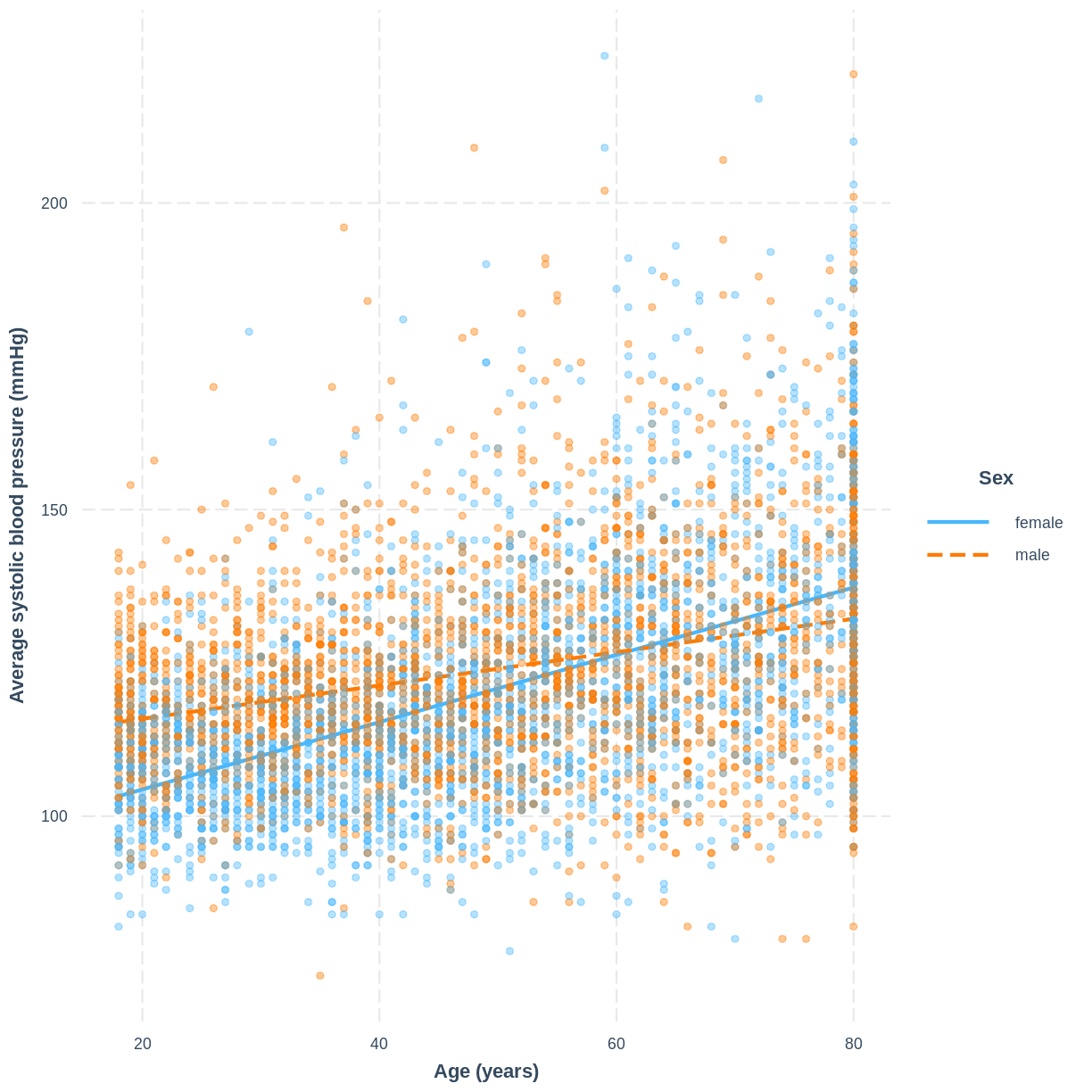
Visualising a multiple linear regression model with an interaction
We can visualise the model, as before, using the interact_plot() function.
interact_plot(BPSysAve_Age_Sex, pred = Age, modx = Sex,
              plot.points = TRUE, point.alpha = 0.4) +
  ylab("Average systolic blood pressure (mmHg)") +
  xlab("Age (years)")
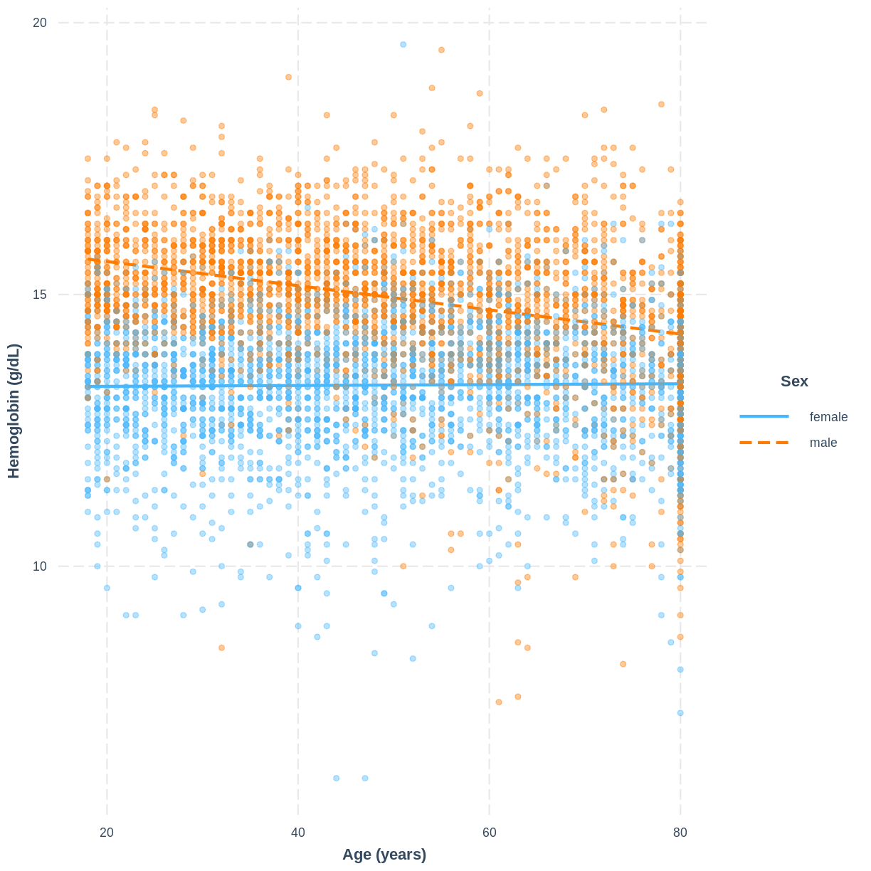
Exercise
To help others interpret the
Hemoglobin_Age_Sexmodel, produce a figure. Make this figure using theinteractionspackage.Solution
interact_plot(Hemoglobin_Age_Sex, pred = Age, modx = Sex,
              plot.points = TRUE, point.alpha = 0.4) +
  ylab("Hemoglobin (g/dL)") +
  xlab("Age (years)")
Key Points
It may be appropriate to include an interaction when the slopes appear to differ across levels of a categorical variable.
Replace
+by*in thelm()command to add an interaction.When an interaction is included, two coefficients relate to differences between the two levels of a categorical variable - one relates to a difference in the intercept, the other to a difference in the slope.
The function
interact_plot()can be used to visualise the model.