Linear regression with one continuous and one categorical explanatory variable

Overview

Teaching: 15 min
Exercises: 20 min

Questions

• How can we visualise the relationship between three variables, two of which are continuous and one of which is categorical, in R?

• How can we fit a linear regression model to this type of data in R?

• How can we obtain and interpret the model parameters?

• How can we visualise the linear regression model in R?

Objectives

• Explore the relationship between a continuous dependent variable and two explanatory variables, one continuous and one categorical, using ggplot2.

• Fit a linear regression model with one continuous explanatory variable and one categorical explanatory variable using lm().

• Use the jtools package to interpret the model output.

• Use the interactions package to visualise the model output.

In this episode we will learn to fit a linear regression model when we have two explanatory variables: one continuous and one categorical. Before we fit the model, we can explore the relationship between our variables graphically. We are asking the question: does the relationship between the continuous explanatory variable and the response variable differ between the levels of the categorical variable?

Exploratory plots

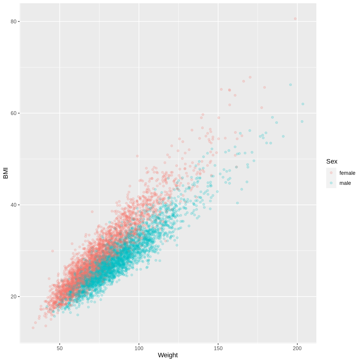
Let us take the response variable BMI, the continuous explanatory variable Weight and the categorical explanatory variable Sex as an example. The code below subsets our data for individuals who are older than 17 years with filter(). The plotting is then initiated using ggplot(). Inside aes(), we select the response variable with y = BMI, the continuous explanatory variable with x = Weight and the categorical explanatory variable with colour = Sex. As a consequence of the final argument, the points produced by geom_point() are coloured by Sex. Finally, we include opacity using alpha = 0.2, which allows us to distinguish areas dense in points from sparser areas. Note that RStudio returns the warning “Removed 320 rows containing missing values (geom_point).” - this reflects that 320 participants had missing BMI and/or Weight data.

The plot suggests that on average, participants classed as female have a higher BMI than participants classed as male, for any particular value of Weight. We might therefore want to account for this in our model by having separate intercepts for the levels of Sex.

dat %>%
  filter(Age > 17) %>%
  ggplot(aes(x = Weight, y = BMI, colour = Sex)) +
  geom_point(alpha = 0.2) 

Exercise

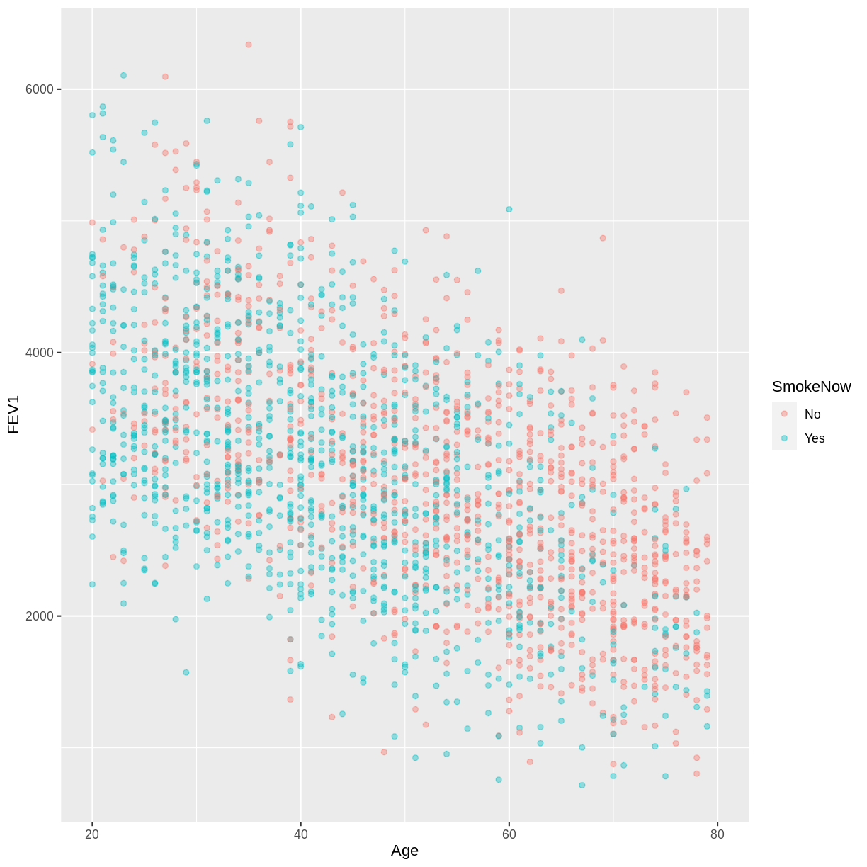
You have been asked to model the relationship between FEV1 and Age in the NHANES data, splitting observations by whether participants are active or ex smokers (SmokeNow). Use the ggplot2 package to create an exploratory plot, ensuring that:

1. NAs are discarded from the SmokeNow variable.
2. FEV1 (FEV1) is on the y-axis and Age (Age) is on the x-axis.
3. These data are shown as a scatterplot, with points coloured by SmokeNow and an opacity of 0.4.

Solution

dat %>%
 drop_na(SmokeNow) %>%
 ggplot(aes(x = Age, y = FEV1, colour = SmokeNow)) +
 geom_point(alpha = 0.4)

Fitting and interpreting a multiple linear regression model

We fit the model using lm(). With formula = BMI ~ Weight + Sex we specify that our model has two explanatory variables, Weight and Sex.

BMI_Weight_Sex <- dat %>%
  filter(Age > 17) %>%
  lm(formula = BMI ~ Weight + Sex)

The linear model equation associated with this model has the general form

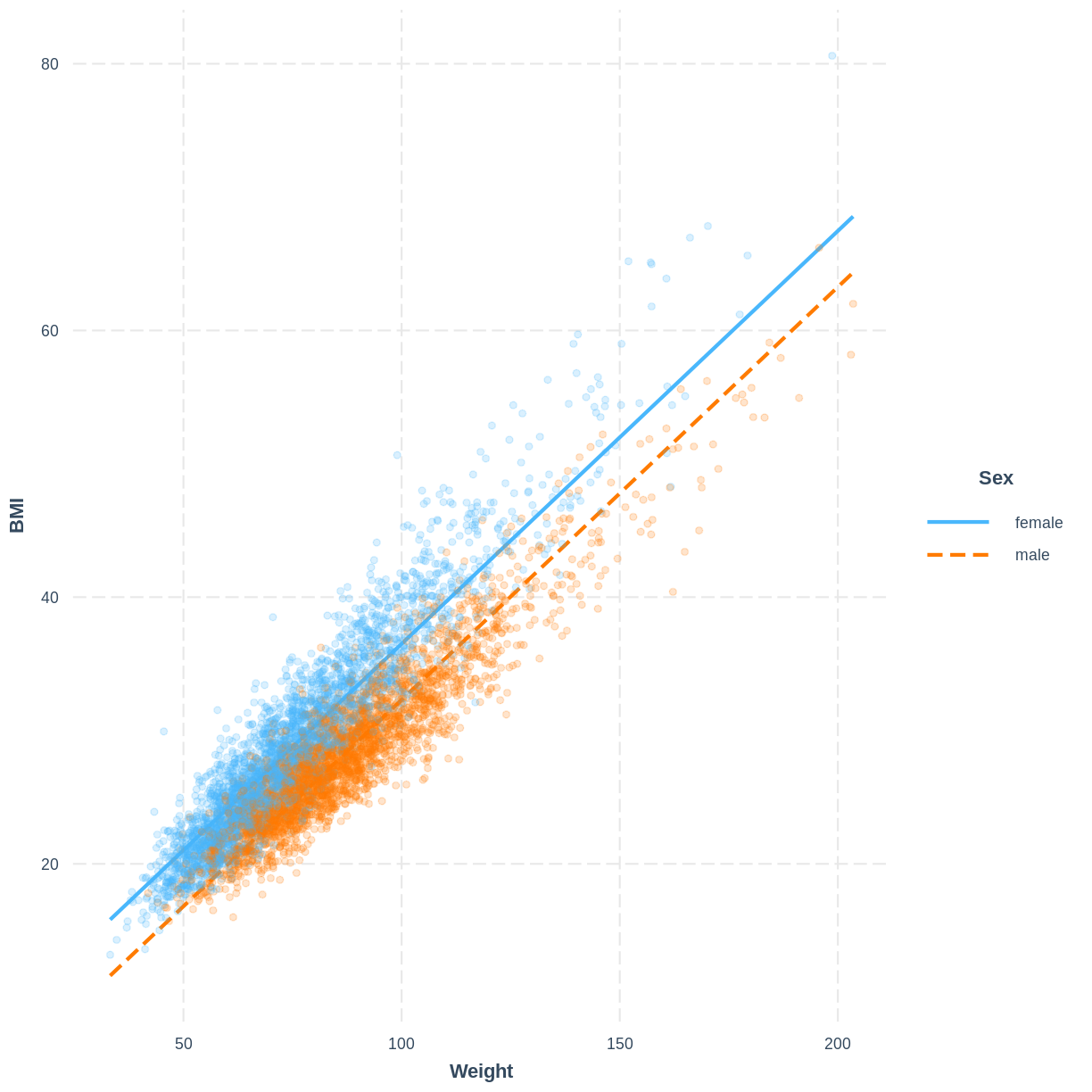
Notice that we now have the additional parameters, $\beta_2$ and $x_2$, in comparison to the simple linear regression model equation. In the context of our model, $\beta_1$ is the parameter for the effect of Weight and $\beta_2$ is the parameter for the effect of Sex. Recall from the simple linear regression lesson that a categorical variable has a baseline level in R. The parameter associated with the categorical variable then estimates the difference in the outcome variable in a group different from the baseline. Since “f” precedes “m” in the alphabet, R takes female as the baseline level. Therefore, $\beta_2$ estimates the difference in BMI between males and females, given a particular value for Weight. $\beta_2$ is only included when $x_2 = 1$, i.e. when the Sex of a participant is male. This results in separate intercepts for the levels of Sex: the intercept for females is given by $\beta_0$ and the intercept for males is given by $\beta_0 + \beta_2$. In this model, the effect of Weight is given by $\beta_1$, irrespective of the Sex of a participant. This results in equal slopes across the levels of Sex.

The model parameters can be obtained using summ() from the jtools package. We include 95% confidence intervals for the parameter estimates using confint = TRUE and three digits after the decimal point using digits = 3. The intercept when Sex = female equals $5.538$ and the intercept when Sex = male equals $5.538 - 4.202 = 1.336$. Notice that in this model, the effect of Weight is $0.310$, regardless of Sex. The model equation can therefore be updated to be:

where $x_2 = 1$ for Sex = male and $0$ otherwise.

summ(BMI_Weight_Sex, confint = TRUE, digits = 3)

MODEL INFO:
Observations: 6177 (320 missing obs. deleted)
Dependent Variable: BMI
Type: OLS linear regression 

MODEL FIT:
F(2,6174) = 19431.981, p = 0.000
R² = 0.863
Adj. R² = 0.863 

Standard errors: OLS
--------------------------------------------------------------
                      Est.     2.5%    97.5%    t val.       p
----------------- -------- -------- -------- --------- -------
(Intercept)          5.538    5.289    5.787    43.656   0.000
Weight               0.310    0.307    0.313   196.965   0.000
Sexmale             -4.202   -4.333   -4.071   -63.075   0.000
--------------------------------------------------------------

Exercise

1. Using the lm() command, fit a multiple linear regression of FEV1 (FEV1) as a function of Age (Age), grouped by SmokeNow. Name this lm object FEV1_Age_SmokeNow.
2. Using the summ function from the jtools package, answer the following questions:

A) What FEV1 does the model predict, on average, for an individual, belonging to the baseline level of SmokeNow, with an Age of 0?
B) What is R taking as the baseline level of SmokeNow and why?
C) By how much is FEV1 expected to differ, on average, between the baseline and the alternative level of SmokeNow?
D) By how much is FEV1 expected to differ, on average, for a one-unit difference in Age?
E) Given these values and the names of the response and explanatory variables, how can the general equation $E(y) = \beta_0 + {\beta}_1 \times x_1 + {\beta}_2 \times x_2$ be adapted to represent the model?

Solution

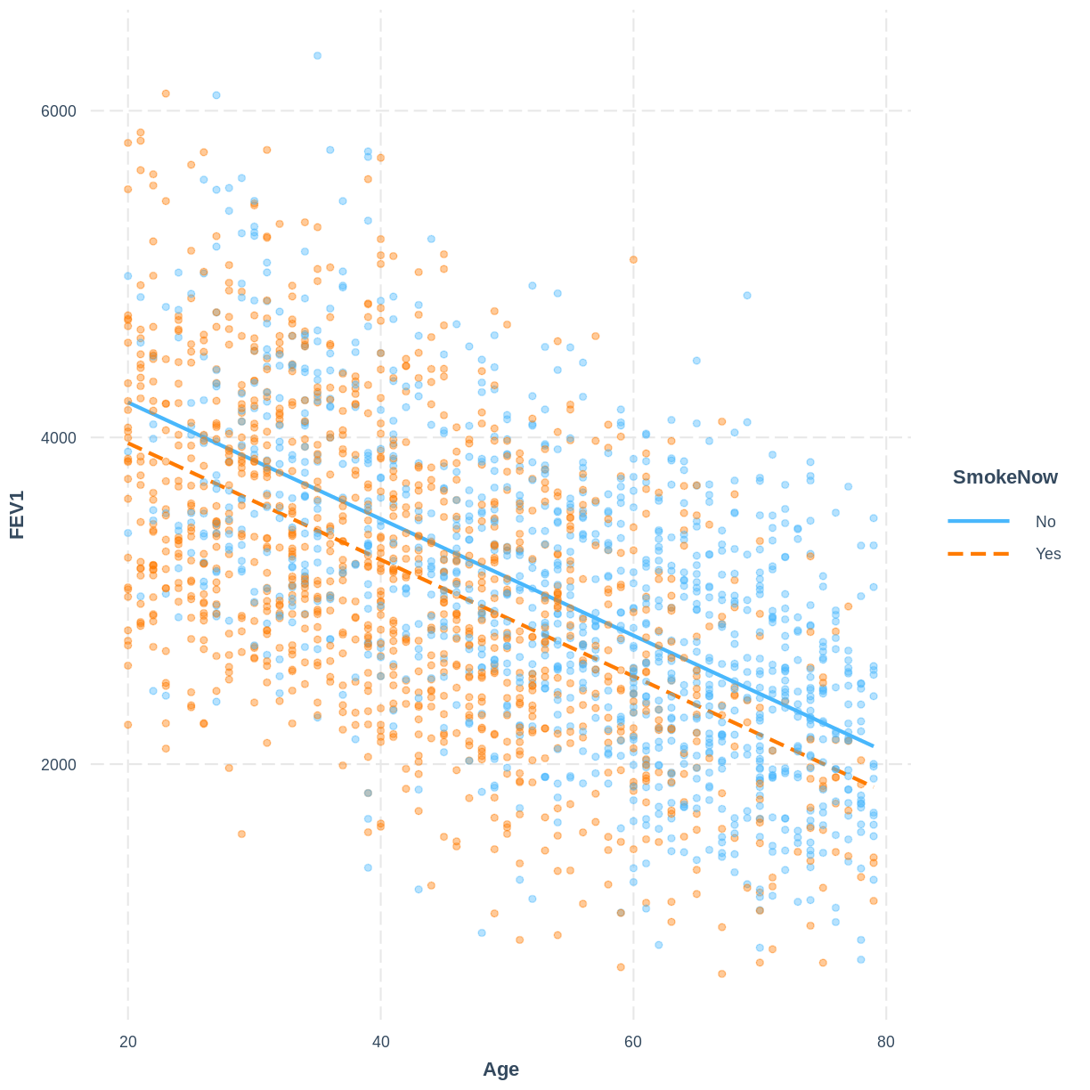
FEV1_Age_SmokeNow <- dat %>%
  lm(formula = FEV1 ~ Age + SmokeNow)

summ(FEV1_Age_SmokeNow, confint = TRUE, digits=3)

MODEL INFO:
Observations: 2265 (7735 missing obs. deleted)
Dependent Variable: FEV1
Type: OLS linear regression 

MODEL FIT:
F(2,2262) = 560.807, p = 0.000
R² = 0.331
Adj. R² = 0.331 

Standard errors: OLS
--------------------------------------------------------------------
                        Est.       2.5%      97.5%    t val.       p
----------------- ---------- ---------- ---------- --------- -------
(Intercept)         4928.155   4805.493   5050.816    78.787   0.000
Age                  -35.686    -37.799    -33.573   -33.117   0.000
SmokeNowYes         -249.305   -317.045   -181.564    -7.217   0.000
--------------------------------------------------------------------

A) 4928.155 mL
B) No, because “n” precedes “y” in the alphabet.
C) On average, individuals from the two categories are expected to differ by 249.305 mL.
D) It is expected to decrease by 35.686 mL.
E) $E(\text{FEV1}) = 4928.155 - 35.686 \times \text{Age} - 249.305 \times x_2$,
where $x_2 = 1$ for current smokers and $0$ otherwise.

Visualising a multiple linear regression model

The model can be visualised using two lines, representing the levels of Sex. Rather than using effect_plot() from the jtools package, we use interact_plot from the interactions package. We specify the model by its name, the continuous explanatory variable using pred = Weight and the categorical explanatory variable using modx = Sex. We include the data points using plot.points = TRUE and introduce opacity into the data points using point.alpha = 0.2.

Note that R returns the warning “Weight and Sex are not included in an interaction with one another in the model.” - we will learn what interactions are and when they might be appropriate in the next episode. In this scenario we can safely ignore the warning.

interact_plot(BMI_Weight_Sex, pred = Weight, modx = Sex,
              plot.points = TRUE, point.alpha = 0.2)

Exercise

To help others interpret the FEV1_Age_SmokeNow model, produce a figure. Make this figure using the interactions package.

Solution

interact_plot(FEV1_Age_SmokeNow, pred = Age, modx = SmokeNow,
              plot.points = TRUE, point.alpha = 0.4)

Key Points

• A scatterplot, with points coloured by the levels of a categorical variable, can be used to explore the relationship between two continuous variables and a categorical variable.

• The categorical variable can be added to the formula in lm() using a +.

• The model output shows separate intercepts for the levels of the categorical variable. The slope across the levels of the categorical variable is held constant.

• Parallel lines can be added to the exploratory scatterplot to visualise the linear regression model.