Trial Design

Overview

Teaching: min
Exercises: min

Questions

• What kind of on-farm experiments do we do?

• How do we design these experiments efficiently?

Objectives

• Know different types of common on-farm experiments

• Import boundary file and AB line file

• Create AB line file with code

• utilize the functions to create simple trial designs

Trial design

To determine the most cost effective seed and fertilizer rates in a given field, we need to figure out:

• How much seed and nitrogen am I applying in this field now?
• How much does seed and nitrogen currently cost me?
• Should I apply more seed and/or nitrogen to improve profits?
• Could I apply less seed and/or nitrogen without reducing profits?
• How do I minimize the cost of inputs (seed and nitrogen) while maximizing yield (bushels per acre) at the current cost of seed and nitrogen?

In order to help figure this out, we create a grid over the field in which we combine areas of high, medium, and low rates of seed and fertilizer independently of each other. Some of the potential variations on this grid include:

• High seed and high fertilizer
• Low seed and high fertilizer
• Low seed and low fertilizer
• Several middle points between any of these combinations

Then we look at differences in yield data in the different areas of the field to determine:

• Whether more seed and more fertilizer made enough of a difference to be significant
• Where the most cost-effective seed and fertilizer rates are at the current prices of seed and nitrogen

For the next step, we will design our own experiments on the sample field. The only files we will need for the trial design are the boundary file and ab line.

Read and transform shape files

We will start by reading in the shape files we need:

boundary <- read_sf("data/boundary.gpkg") # read in boundary
abline <- read_sf("data/abline.gpkg") # read in AB line

Now let’s check the coordinate references of our two files:

st_crs(boundary)

Coordinate Reference System:
  EPSG: 4326 
  proj4string: "+proj=longlat +datum=WGS84 +no_defs"

st_crs(abline)

Coordinate Reference System:
  EPSG: 4326 
  proj4string: "+proj=longlat +datum=WGS84 +no_defs"

Since both of these are in lat/long and we want them in UTM, we’ll transform them:

trialarea <- st_transform_utm(boundary)
abline_utm <- st_transform_utm(abline)

Designing trials

We need decide on the details of experiment design before we get into any of the code. Relative parameters we need for the trial design include:

• plot dimensions
• number of treatments
• types of treatments, and
• treatment range.

Defining Parameters

In the following code, we are simply going to assign values to all the parameters that might be involved in the trial design. In this way, if we ever want to change any parameters, we can do it here, and need not to worry about the consistency for the whole code.

Now let’s design our grid with the following parameters:

width_in_meters <- 24 # width of grids is 24 meters
long_direction <- 'NS' # direction of grid that will be long in relation to AB line
short_direction <- 'EW' # direction of grid that will be short in relation to AB line
length_in_ft <- 180 # length of grids in feet

Make Grids

We’ll use our make_grids again function to generate this trial’s grid:

width <- m_to_ft(24) # convert meters to feet
design_grids_utm <- make_grids(trialarea, abline_utm,
             long_in = long_direction,
			       short_in = short_direction,
			       length_ft = length_in_ft,
			       width_ft = width)

Next we want to make sure the coordinate reference frame of our trialarea is the same as our design_grids_utm grids and then take the intersection of these grids with our trial area as we did previously:

st_crs(design_grids_utm) <- st_crs(trialarea)
trial_grid <- st_intersection(trialarea, design_grids_utm)

Warning: attribute variables are assumed to be spatially constant throughout all
geometries

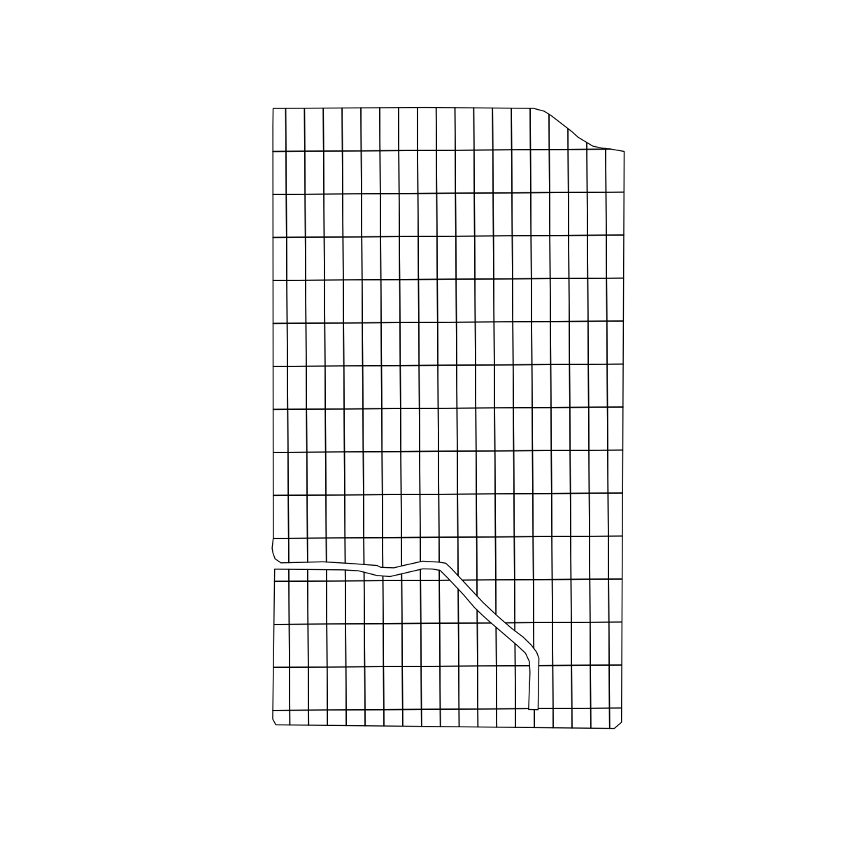
Let’s check out what our trial subplots look like:

plot(trial_grid$geom)

Determining subplot treatments

Now that we have the trial design plots, we need to assign different treatments to each plot. We can use the treat_assign function from functions.R to randomly assign seed rates and nitrogen rates to each plot on our grid.

We’ll select 4 different seed rates and 4 different nitrogen rates to deposit randomly on our grid:

seed_rates <- c(31000, 34000, 37000, 40000)
nitrogen_rates <- c(160,200,225,250)

The seed_quo and nitrogen_quo are the rates that will be applied to the headlands that are not part of the trial.

seed_quo <- 37000
nitrogen_quo <- 225

Lists of elements in R

You’ll see this definition of a list of numbers (or text) in R with a c(). This is just a special way of saying all the elements in this list “belong” together, like with all of the numbers in a column of a spreadsheet “belonging” together.

Generating Treatment Map

We are now ready to generate our treatment plot:

whole_plot <- treat_assign(trialarea, trial_grid, head_buffer_ft = width,
                           seed_treat_rates = seed_rates,
			   nitrogen_treat_rates = nitrogen_rates,
			   seed_quo = seed_quo,
			   nitrogen_quo = nitrogen_quo,
			   set_seed=TRUE)

Simulating yields

Because you are generating your trial design “on the fly” in this workshop you will have different nitrogen and seed application rates than for the original dataset which measured the yields from a “real” trial. Because we want everybody to be using the same trial data we have set a flag set_seed=TRUE in our call to treat_assign. When you do this on your own you can set this parameter to FALSE or just leave it out of the function call altogether.

Mapping Trials

Let’s look at what our trial looks like. First, as a shape file:

head(whole_plot)

Simple feature collection with 6 features and 4 fields
geometry type:  POLYGON
dimension:      XY
bbox:           xmin: 342043.5 ymin: 4523203 xmax: 342066.9 ymax: 4523349
epsg (SRID):    32617
proj4string:    +proj=utm +zone=17 +datum=WGS84 +units=m +no_defs
# A tibble: 6 x 5
  id    treat_type NRATE SEEDRATE                                           geom
  <chr>      <dbl> <dbl>    <dbl>                                  <POLYGON [m]>
1 ID1           17   225    37000 ((342066.7 4523313, 342043.7 4523313, 342043.…
2 ID2           17   225    37000 ((342066.7 4523313, 342043.7 4523313, 342043.…
3 ID3            5   200    31000 ((342066.5 4523258, 342044.1 4523258, 342043.…
4 ID4            2   160    34000 ((342066.5 4523258, 342044.1 4523258, 342043.…
5 ID5           16   250    40000 ((342066.2 4523203, 342044.5 4523203, 342044.…
6 ID6            7   200    37000 ((342066.2 4523203, 342044.5 4523203, 342044.…

Or, we can look at the plots one at a time using a map_poly function from functions.R. For the seeding rate:

seed_plot <- map_poly(whole_plot, "SEEDRATE", "Seedrate Treatment")
seed_plot # to show our plot

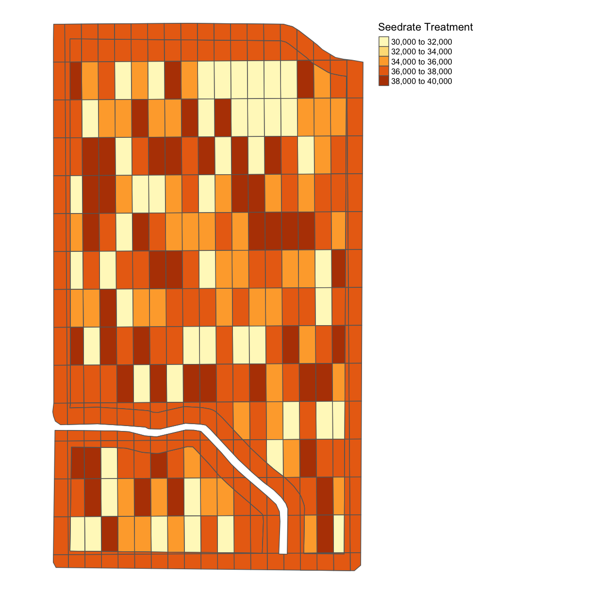Here, we give map_poly our whole_plot geometry variable, what variable we want to show, in the above case, SEEDRATE, and the label to our legend, here Seedrate Treatement.

We can also plot the nitrogen application rate:

nitrogen_plot <- map_poly(whole_plot, "NRATE", "Nitrogen Treatment")
nitrogen_plot

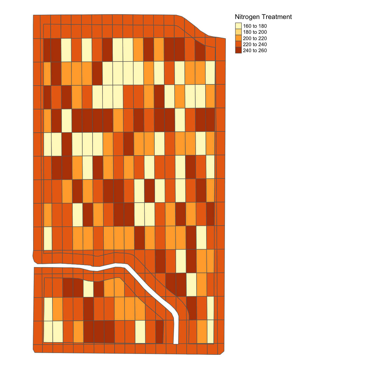
We can also use the function tmap_arrange to show these plots side-by-side;

nitrogen_plot <- map_poly(whole_plot, "NRATE", "Nitrogen Treatment")
seed_plot <- map_poly(whole_plot, "SEEDRATE", "Seedrate Treatment")
treatment_plot_comp <- tmap_arrange(nitrogen_plot, seed_plot, ncol = 2, nrow = 1)
treatment_plot_comp

Key Points

• Most of the code in this part would be using the functions, therefore understanding what different functions can be quite important

• In designing the trials, the most important thing is to know how to design the experimental rates,and the tech part can be done by someone else