Geospatial data and boundaries
Overview
Teaching: min
Exercises: minQuestions
How do I read shape files into R?
What is a coordinate reference system (CRS)?
What is my shape file’s coordinate reference system?
Objectives
Import geospatial files into your R environment
Identify the coordinate system for a dataset
Talk about when data don’t have a projection defined (missing
.prjfile)Determine UTM zone of a dataset
Reproject the dataset into UTM
Visualize geospatial data with R
Introducing Spatial Data
Spatial data can be stored in many different ways, and an important part of using your farm’s data will involve understanding what format your data is already in and what format another program needs it to be in. During the course of this lesson, we’ll learn:
- How to identify which coordinate reference system (CRS) a data file is using
- How, when, and why to transform data from the WGS84 standard to the UTM standard (or vice versa)
- How to save the transformed data as a new file
- Some ways of creating visualizations from your data
What is a CRS?
Geospatial data has a coordinate reference system (CRS) that reports how the map is projected and what point is used as a reference. A projection is a way of making the earth’s curved surface fit into something you can represent on a flat computer screen. The point used for reference during projection is called a datum.
Importance of Projections
When you cut an orange, it’s impossible to get the peel to lay flat (without really smashing it). The Earth, of course, behaves similarly, leading to distortion in the map. The kind of distortion can be chosen by using a different projection, or mathematical scheme for converting the round Earth to a flat map.
To understand how much projection matters, take a look at the difference between the Mercator projection of the world and the Boggs eumorphic projection.
| Mercator | Boggs eumorphic projection |
|---|---|
 |
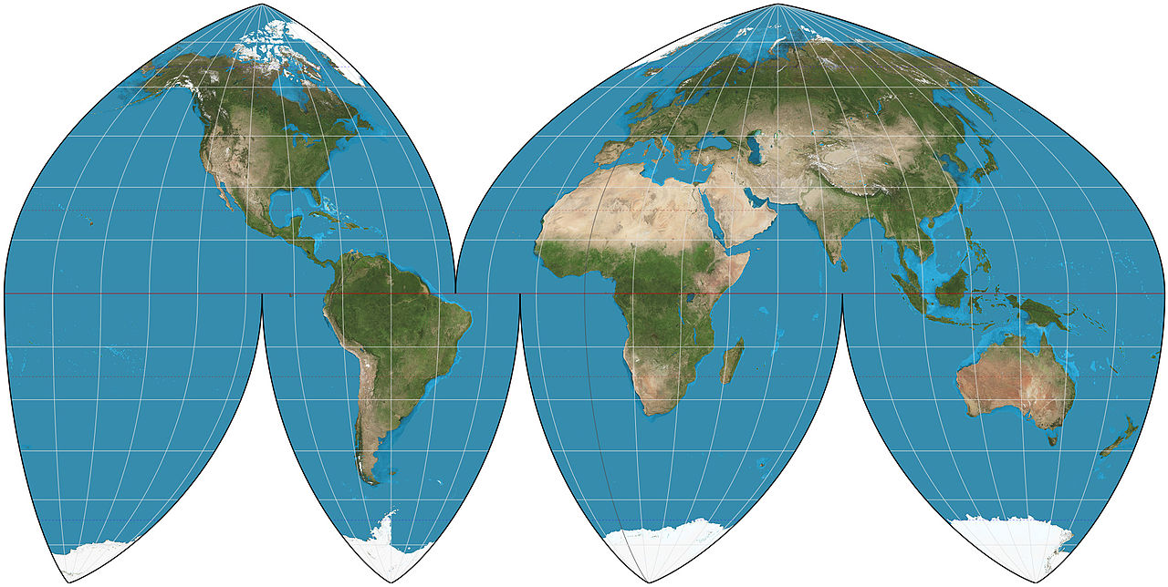 |
In the Mercator projection, space that doesn’t exist is created to make a “flat” map. Greenland and Antarctica wind up disproportionately huge. In the Boggs projection, strategic slices are cut out of the ocean so that the sizes appear a bit closer to true, but Canada and Russia get pinched and Greenland gets bisected. There will always be some compromises made in a projection system that converts curved surfaces to flat ones for the same reason that it’s difficult to make an orange peel lie flat. So the method you select will have an effect on your outcome.
Understanding file types and CRS types
Geospatial data files have several potential variations, including:
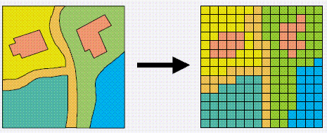
- Vector or raster data: Whether the information is stored as lines and curves (vector) or as individual dots (raster or bitmap).
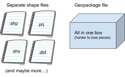
- File types: Several different shape files or one unified geopackage file
- Coordinate reference systems (CRSes): Latitude/longitude (WGS84, measured in degrees) or UTM (measured as a distance from a fixed point in meters)
Any of this information can come in any combination – you can have vector or raster data in any CRS in either a geopackage file or a collection of shape files.
The image on the left below is a vector-based representation of GIS data, with lines and curves; the image on the right is a raster-based representation, with individual values assigned to particular locations in a grid.
In order to make data from different sources work together, you’ll need to be able to identify what type of data in what CRS you have and how to convert them to the same type of thing—making sure you’re comparing apples to apples.
For example:
- The data coming from your equipment will probably be in separate shape files. This allows the steering system to work with one file, the planting system to track rates in another file, and so forth. It’s like giving a group of reporters their own notebooks, instead of asking them all to share the same notebook at the same time.
- However, once the data has been collected, it’s easier for us to combine those reporters’ notebooks into one
geopackagefile so that the data is all in one place for us to work with at the same time. - Data coming from your equipment will also likely be reported in a CRS based on latitude/longitude (WGS84), but in order to do calculations based on distance within a field, we’ll want to convert to UTM.
- Because each equipment manufacturer has their own standards, there may be some additional manipulation needed to get from the manufacturer’s possibly proprietary standard to something that you can use yourself. (This is one reason it’s helpful to provide us with data before class begins, so that we can help work out the pattern for decoding your equipment manufacturer’s data before the workshop starts.)
Loading Libraries
In the beginning of this workshop, we had you all install a bunch of packages that have a collection of functions we are going to use to plot our data. We want to tell R to load in all of these functions, and we can do that by using the library function:
library("rgdal")
library("plyr")
library("dplyr")
library("sp")
library("sf")
library("gstat")
library("tmap")
library("measurements")
library("daymetr")
library("FedData")
library("lubridate")
library("raster")
library("data.table")
library("broom")
library("ggplot2")

# load functions for this workshop
source('https://raw.githubusercontent.com/data-carpentry-for-agriculture/trial-lesson/gh-pages/_episodes_rmd/functions.R')

# you need your specific working directory here with something like:
#setwd(YOUR DIR)
This should generate a lot of output, and some of it will be warnings (in red), but that is to be expected.
Reading in the Boundary File
Before we can look at a CRS in R, we need to have a geospatial file in the R environment. We will bring in the field boundary. Use the function read_sf() to bring the dataset into your R environment. Because we have already set the working directory for this file, we don’t need to give the whole path, just the folder data that the gpkg file is stored within.
boundary <- read_sf("data/boundary.gpkg")
There are many functions for reading files into the environment, but read_sf() creates an object of class sf (simple feature). This class makes accessing spatial data much easier. Much like a data frame, you can access variables within an sf object using the $ operator. For this and other reasons like the number of spatial calculations available for sf objects, this class is perferred in most situations.
Check the coordinate reference system
The function for retreiving the CRS of a simple feature is st_crs(). Generally it is good practice to know the CRS of your files, but it becomes critical when combining files and performing operations on geospatial data. Some commands will not work if the data is in the wrong CRS or if two dataframes are in different CRSs.
st_crs(boundary)
Coordinate Reference System:
  EPSG: 4326
  proj4string: "+proj=longlat +datum=WGS84 +no_defs"
The boundary file is projected in longitude and latitude using the WGS84 datum. This will be the CRS of most of the data you see.
Lost
.prjfilesSometimes when looking at a shapefile, the
.prjfile may be lost. Thenst_crs()will return empty, butsfobjects still contain a geometry columngeom. We can see the geometric points for the vertices of each polygon or the points in the data.head(boundary$geom)Geometry set for 1 feature geometry type: POLYGON dimension: XY bbox: xmin: -82.87853 ymin: 40.83945 xmax: -82.87306 ymax: 40.8466 epsg (SRID): 4326 proj4string: +proj=longlat +datum=WGS84 +no_defsPOLYGON ((-82.87319 40.84574, -82.87306 40.8398...
UTM Zones
Some coordinate reference systems, such as UTM zones, are measured in meters. Latitude and longitude represent a different type of CRS, defined in terms of angles across a sphere. If we want to create measures of distance, we need the trial design in UTM. But there are many UTM zones, so we must determine the zone of the trial area.
The UTM system divides the surface of Earth between 80°S and 84°N latitude into 60 zones, each 6° of longitude in width. Zone 1 covers longitude 180° to 174° W; zone numbering increases eastward to zone 60 that covers longitude 174 to 180 East.

st_transform and ESPG Codes
For reprojecting spatial data, the function st_transform() uses an ESPG code to transform a simple feature to the new CRS. The ESPG Geodetic Parameter Dataset is a public registry of spatial reference systems, Earth ellipsoids, coordinate transformations and related units of measurement. The ESPG is one way to assign or transform the CRS in R.
The ESPG for UTM always begins with “326” and the last numbers are the number of the zone. The ESPG for WGS84 is 4326. This is the projection your equipment reads, so any trial design files will need to be transformed back into WGS84 before you implement the trial. Also, all files from your machinery, such as yield, as-applied, and as-planted, will be reported in latitude and longitude with WGS84.
Transforming
The function st_transform_utm() transforms a simple feature that is in lat/long into UTM. This function is in the functions.R script, and is described there in more detail. Make sure that you have run source("functions.R") or you will not have the function in your global environment.
boundaryutm <- st_transform_utm(boundary)
st_crs(boundaryutm)
Joint Exercise: Exploring Geospatial Files
Instructors: ask the students how to do this first, then type along with explanation.
- Bring the file called
"asplanted.gpkg"(from thedatasubdirectory of yourWorkingDir) in your environment. Name the objectplanting. This file contains the planting information for 2017.- Identify the CRS of the object.
- Look at the geometry features. What kind of geometric features are in this dataset?
- Transform the file to UTM or Lat/Long, depending on the current CRS.
Solution
planting <- read_sf("data/asplanted.gpkg")
st_crs(planting)
Coordinate Reference System: EPSG: 4326 proj4string: "+proj=longlat +datum=WGS84 +no_defs"planting$geomGeometry set for 6382 features geometry type: POINT dimension: XY bbox: xmin: -82.87843 ymin: 40.83952 xmax: -82.87315 ymax: 40.84653 epsg (SRID): 4326 proj4string: +proj=longlat +datum=WGS84 +no_defs First 5 geometries:POINT (-82.87829 40.83953)POINT (-82.87828 40.83953) POINT (-82.87828 40.83953)POINT (-82.87827 40.83953)POINT (-82.87825 40.83953)plantingutm <- st_transform_utm(planting) st_crs(plantingutm)Coordinate Reference System: EPSG: 32617 proj4string: "+proj=utm +zone=17 +datum=WGS84 +units=m +no_defs"
Exercise Discussion
The cleaned planting file was in WGS84 initially. When we look at the geometry features, they are 6382 points defined in xand y coordinates. Using st_transform_utm() we create a new file called plantingutm with the CRS of UTM zone 17.
Save the file
Use st_write() to save an sf object. If you do not specify a directory, the working directory will be used. We include the object we are saving boundaryutm and the name we would like to give the saved file "boundary_utm.gpkg". Additionally, we specify the layer_options and update values to enable overwriting an existing file with the same name.
st_write(boundaryutm, "boundary_utm.gpkg", layer_options = 'OVERWRITE=YES')
Error in st_write(boundaryutm, "boundary_utm.gpkg", layer_options = "OVERWRITE=YES"): object 'boundaryutm' not found
The new .gpkg file will be visible in your working directory. (Check it out: Browse to your working directory in Windows File Explorer or Mac Finder and see the date and time on your new file.)
.gpkgvs..shpfilesYou can save the file as a
.gpkgor.shpfile.The advantage of a
.gpkgfile is that you only save one file rather than four files in a shapefile. Because shapefiles contain multiple files, they can be corrupted if one piece is missing. One example is a.prjfile. If the.prjfile is missing, the shapefile will have no CRS, and you will need to determine the CRS of the object. You will often need to transform a file from UTM to lat/long and save the new file during trial design, so this is an important step. One common problem with these files is that when you try to open a.gpkgfile for the first time in R, it might not work if you haven’t opened it in QGIS before.
Visualizing the data
There are several ways to visualize spatial data. One way is to use plot() to look at the basic shape of the data:
plot(boundary$geom)

Data Types
There are many different geospatial data file types in use, which can make processing a bit complicated. We have stuck to using gpkg in our work here because we feel there are fewer ways for the data to get corrupted (as by a lost shp file, for instance). Some other types you may see include:
-
shp. Mentioned a moment ago as having several files to track, theshpformat generates some required files and some optional files.Required files include:
shp, the geometry itselfshx, the shape index filesbf, the attribute formats for each shape
Optional files which may be included are:
cpg, the code page (or encoding) used with thedbffileprj, the project description and CRSsbn,sbx, spatial indices of features
-
geojson. This is a plain text format which is quite flexible. -
tif. This is a graphics file format which has been adapted for storing coordinate reference data with raster images.
Key Points
It is preferred to use
sffor data analysis, making it easier to access the dataframe.Projecting your data in utm is necessary for many of the geometric operations you perform (e.g. making trial grids and splitting plots into subplot data)
Different data formats that you are likely to encounter include
gpkg,shp(cpg,dbf,prj,sbn,sbx),geojson, andtif.