All in One View
Content from Data organisation with spreadsheets
Last updated on 2026-07-14 | Edit this page
Overview
Questions
- How to organise tabular data?
Objectives
- Learn about spreadsheets, their strengths and weaknesses.
- How do we format data in spreadsheets for effective data use?
- Learn about common spreadsheet errors and how to correct them.
- Organise your data according to tidy data principles.
- Learn about text-based spreadsheet formats such as the comma-separated (CSV) or tab-separated (TSV) formats.
This episode is based on the Data Carpentries’s Data Analysis and Visualisation in R for Ecologists lesson.
Spreadsheet programs
Question
- What are basic principles for using spreadsheets for good data organization?
Objective
- Describe best practices for organizing data so computers can make the best use of datasets.
Keypoint
- Good data organization is the foundation of any research project.
Good data organization is the foundation of your research project. Most researchers have data or do data entry in spreadsheets. Spreadsheet programs are very useful graphical interfaces for designing data tables and handling very basic data quality control functions. See also @Broman:2018.
Spreadsheet outline
Spreadsheets are good for data entry. Therefore we have a lot of data in spreadsheets. Much of your time as a researcher will be spent in this ‘data wrangling’ stage. It’s not the most fun, but it’s necessary. We’ll teach you how to think about data organization and some practices for more effective data wrangling.
What this lesson will not teach you
- How to do statistics in a spreadsheet
- How to do plotting in a spreadsheet
- How to write code in spreadsheet programs
If you’re looking to do this, a good reference is Head First Excel, published by O’Reilly.
Why aren’t we teaching data analysis in spreadsheets
Data analysis in spreadsheets usually requires a lot of manual work. If you want to change a parameter or run an analysis with a new dataset, you usually have to redo everything by hand. (We do know that you can create macros, but see the next point.)
It is also difficult to track or reproduce statistical or plotting analyses done in spreadsheet programs when you want to go back to your work or someone asks for details of your analysis.
Many spreadsheet programs are available. Since most participants utilise Excel as their primary spreadsheet program, this lesson will make use of Excel examples. A free spreadsheet program that can also be used is LibreOffice. Commands may differ a bit between programs, but the general idea is the same.
Spreadsheet programs encompass a lot of the things we need to be able to do as researchers. We can use them for:
- Data entry
- Organizing data
- Subsetting and sorting data
- Statistics
- Plotting
Spreadsheet programs use tables to represent and display data. Data formatted as tables is also the main theme of this chapter, and we will see how to organise data into tables in a standardised way to ensure efficient downstream analysis.
Challenge: Discuss the following points with your neighbour
- Have you used spreadsheets, in your research, courses, or at home?
- What kind of operations do you do in spreadsheets?
- Which ones do you think spreadsheets are good for?
- Have you accidentally done something in a spreadsheet program that made you frustrated or sad?
Problems with spreadsheets
Spreadsheets are good for data entry, but in reality we tend to use spreadsheet programs for much more than data entry. We use them to create data tables for publications, to generate summary statistics, and make figures.
Generating tables for publications in a spreadsheet is not optimal - often, when formatting a data table for publication, we’re reporting key summary statistics in a way that is not really meant to be read as data, and often involves special formatting (merging cells, creating borders, making it pretty). We advise you to do this sort of operation within your document editing software.
The latter two applications, generating statistics and figures, should be used with caution: because of the graphical, drag and drop nature of spreadsheet programs, it can be very difficult, if not impossible, to replicate your steps (much less retrace anyone else’s), particularly if your stats or figures require you to do more complex calculations. Furthermore, in doing calculations in a spreadsheet, it’s easy to accidentally apply a slightly different formula to multiple adjacent cells. When using a command-line based statistics program like R or SAS, it’s practically impossible to apply a calculation to one observation in your dataset but not another unless you’re doing it on purpose.
Using spreadsheets for data entry and cleaning
In this lesson, we will assume that you are most likely using Excel as your primary spreadsheet program - there are others (gnumeric, Calc from OpenOffice), and their functionality is similar, but Excel seems to be the program most used by biologists and biomedical researchers.
In this lesson we’re going to talk about:
- Formatting data tables in spreadsheets
- Formatting problems
- Exporting data
Formatting data tables in spreadsheets
Questions
- How do we format data in spreadsheets for effective data use?
Objectives
Describe best practices for data entry and formatting in spreadsheets.
Apply best practices to arrange variables and observations in a spreadsheet.
Keypoints
Never modify your raw data. Always make a copy before making any changes.
Keep track of all of the steps you take to clean your data in a plain text file.
Organise your data according to tidy data principles.
The most common mistake made is treating spreadsheet programs like lab notebooks, that is, relying on context, notes in the margin, spatial layout of data and fields to convey information. As humans, we can (usually) interpret these things, but computers don’t view information the same way, and unless we explain to the computer what every single thing means (and that can be hard!), it will not be able to see how our data fits together.
Using the power of computers, we can manage and analyse data in much more effective and faster ways, but to use that power, we have to set up our data for the computer to be able to understand it (and computers are very literal).
This is why it’s extremely important to set up well-formatted tables from the outset - before you even start entering data from your very first preliminary experiment. Data organization is the foundation of your research project. It can make it easier or harder to work with your data throughout your analysis, so it’s worth thinking about when you’re doing your data entry or setting up your experiment. You can set things up in different ways in spreadsheets, but some of these choices can limit your ability to work with the data in other programs or have the you-of-6-months-from-now or your collaborator work with the data.
Note: the best layouts/formats (as well as software and interfaces) for data entry and data analysis might be different. It is important to take this into account, and ideally automate the conversion from one to another.
Keeping track of your analyses
When you’re working with spreadsheets, during data clean up or analyses, it’s very easy to end up with a spreadsheet that looks very different from the one you started with. In order to be able to reproduce your analyses or figure out what you did when a reviewer or instructor asks for a different analysis, you should
create a new file with your cleaned or analysed data. Don’t modify the original dataset, or you will never know where you started!
keep track of the steps you took in your clean up or analysis. You should track these steps as you would any step in an experiment. We recommend that you do this in a plain text file stored in the same folder as the data file.
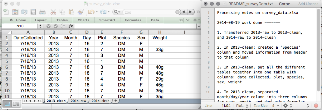
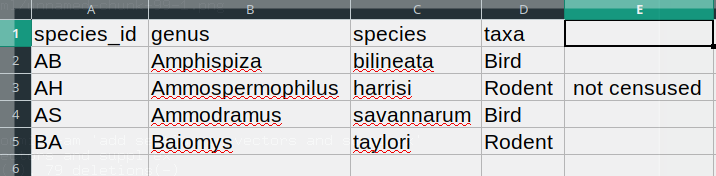
This might be an example of a spreadsheet setup:
Put these principles into practice today during your exercises.
While versioning is out of scope for this course, you can look at the Carpentries lesson on ‘Git’ to learn how to maintain version control over your data. See also this blog post for a quick tutorial or @Perez-Riverol:2016 for a more research-oriented use-case.
Structuring data in spreadsheets
The cardinal rules of using spreadsheet programs for data:
- Put all your variables in columns - the thing you’re measuring, like ‘weight’ or ‘temperature’.
- Put each observation in its own row.
- Don’t combine multiple pieces of information in one cell. Sometimes it just seems like one thing, but think if that’s the only way you’ll want to be able to use or sort that data.
- Leave the raw data raw - don’t change it!
- Export the cleaned data to a text-based format like CSV (comma-separated values) format. This ensures that anyone can use the data, and is required by most data repositories.
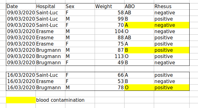
For instance, we have data from patients that visited several hospitals in Brussels, Belgium. They recorded the date of the visit, the hospital, the patients’ gender, weight and blood group.
If we were to keep track of the data like this:
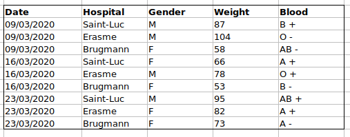
the problem is that the ABO and Rhesus groups are in the same
Blood type column. So, if they wanted to look at all
observations of the A group or look at weight distributions by ABO
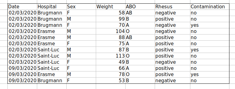
group, it would be tricky to do this using this data setup. If instead
we put the ABO and Rhesus groups in different columns, you can see that
it would be much easier.
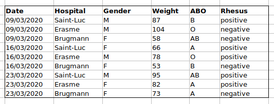
An important rule when setting up a datasheet, is that columns are used for variables and rows are used for observations:
- columns are variables
- rows are observations
- cells are individual values
Challenge: We’re going to take a messy dataset and describe how we would clean it up.
Download a messy dataset by clicking this link.
Open up the data in a spreadsheet program.
You can see that there are two tabs. The data contains various clinical variables recorded in various hospitals in Brussels during the first and second COVID-19 waves in 2020. As you can see, the data have been recorded differently during the March and November waves. Now you’re the person in charge of this project and you want to be able to start analyzing the data.
With the person next to you, identify what is wrong with this spreadsheet. Also discuss the steps you would need to take to clean up first and second wave tabs, and to put them all together in one spreadsheet.
Important: Do not forget our first piece of advice: to create a new file (or tab) for the cleaned data, never modify your original (raw) data.
After you go through this exercise, we’ll discuss as a group what was wrong with this data and how you would fix it.
Challenge: Once you have tidied up the data, answer the following questions:
- How many men and women took part in the study?
- How many A, AB, and B types have been tested?
- As above, but disregarding the contaminated samples?
- How many Rhesus + and - have been tested?
- How many universal donors (O-) have been tested?
- What is the average weight of AB men?
- How many samples have been tested in the different hospitals?
An excellent reference, in particular with regard to R scripting is the Tidy Data paper @Wickham:2014.
Common spreadsheet errors
Questions
- What are some common challenges with formatting data in spreadsheets and how can we avoid them?
Objectives
- Recognise and resolve common spreadsheet formatting problems.
Keypoints
- Avoid using multiple tables within one spreadsheet.
- Avoid spreading data across multiple tabs.
- Record zeros as zeros.
- Use an appropriate null value to record missing data.
- Don’t use formatting to convey information or to make your spreadsheet look pretty.
- Place comments in a separate column.
- Record units in column headers.
- Include only one piece of information in a cell.
- Avoid spaces, numbers and special characters in column headers.
- Avoid special characters in your data.
- Record metadata in a separate plain text file.
There are a few potential errors to be on the lookout for in your own data as well as data from collaborators or the Internet. If you are aware of the errors and the possible negative effect on downstream data analysis and result interpretation, it might motivate yourself and your project members to try and avoid them. Making small changes to the way you format your data in spreadsheets, can have a great impact on efficiency and reliability when it comes to data cleaning and analysis.
- Using multiple tables
- Using multiple tabs
- Not filling in zeros
- Using problematic null values
- Using formatting to convey information
- Using formatting to make the data sheet look pretty
- Placing comments or units in cells
- Entering more than one piece of information in a cell
- Using problematic field names
- Using special characters in data
- Inclusion of metadata in data table
Using multiple tables
A common strategy is creating multiple data tables within one spreadsheet. This confuses the computer, so don’t do this! When you create multiple tables within one spreadsheet, you’re drawing false associations between things for the computer, which sees each row as an observation. You’re also potentially using the same field name in multiple places, which will make it harder to clean your data up into a usable form. The example below depicts the problem:
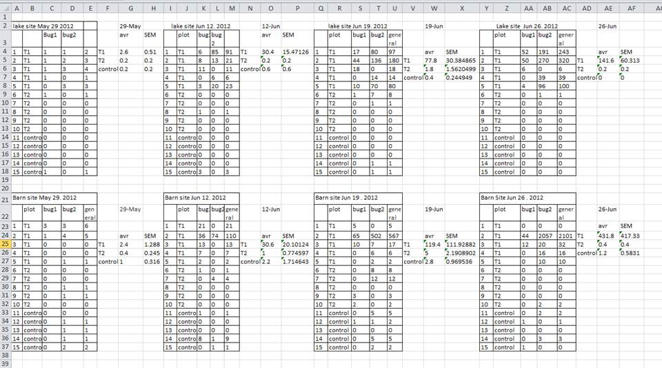
In the example above, the computer will see (for example) row 4 and assume that all columns A-AF refer to the same sample. This row actually represents four distinct samples (sample 1 for each of four different collection dates - May 29th, June 12th, June 19th, and June 26th), as well as some calculated summary statistics (an average (avr) and standard error of measurement (SEM)) for two of those samples. Other rows are similarly problematic.
Using multiple tabs
But what about workbook tabs? That seems like an easy way to organise data, right? Well, yes and no. When you create extra tabs, you fail to allow the computer to see connections in the data that are there (you have to introduce spreadsheet application-specific functions or scripting to ensure this connection). Say, for instance, you make a separate tab for each day you take a measurement.
This isn’t good practice for two reasons:
you are more likely to accidentally add inconsistencies to your data if each time you take a measurement, you start recording data in a new tab, and
even if you manage to prevent all inconsistencies from creeping in, you will add an extra step for yourself before you analyse the data because you will have to combine these data into a single datatable. You will have to explicitly tell the computer how to combine tabs - and if the tabs are inconsistently formatted, you might even have to do it manually.
The next time you’re entering data, and you go to create another tab or table, ask yourself if you could avoid adding this tab by adding another column to your original spreadsheet. We used multiple tabs in our example of a messy data file, but now you’ve seen how you can reorganise your data to consolidate across tabs.
Your data sheet might get very long over the course of the experiment. This makes it harder to enter data if you can’t see your headers at the top of the spreadsheet. But don’t repeat your header row. These can easily get mixed into the data, leading to problems down the road. Instead you can freeze the column headers so that they remain visible even when you have a spreadsheet with many rows.
Not filling in zeros
It might be that when you’re measuring something, it’s usually a zero, say the number of times a rabbit is observed in the survey. Why bother writing in the number zero in that column, when it’s mostly zeros?
However, there’s a difference between a zero and a blank cell in a spreadsheet. To the computer, a zero is actually data. You measured or counted it. A blank cell means that it wasn’t measured and the computer will interpret it as an unknown value (also known as a null or missing value).
The spreadsheets or statistical programs will likely misinterpret blank cells that you intend to be zeros. By not entering the value of your observation, you are telling your computer to represent that data as unknown or missing (null). This can cause problems with subsequent calculations or analyses. For example, the average of a set of numbers which includes a single null value is always null (because the computer can’t guess the value of the missing observations). Because of this, it’s very important to record zeros as zeros and truly missing data as nulls.
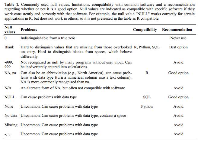
Using problematic null values
Example: using -999 or other numerical values (or zero) to represent missing data.
Solutions:
There are a few reasons why null values get represented differently within a dataset. Sometimes confusing null values are automatically recorded from the measuring device. If that’s the case, there’s not much you can do, but it can be addressed in data cleaning with a tool like OpenRefine before analysis. Other times different null values are used to convey different reasons why the data isn’t there. This is important information to capture, but is in effect using one column to capture two pieces of information. Like for using formatting to convey information it would be good here to create a new column like ‘data_missing’ and use that column to capture the different reasons.
Whatever the reason, it’s a problem if unknown or missing data is recorded as -999, 999, or 0.
Many statistical programs will not recognise that these are intended to represent missing (null) values. How these values are interpreted will depend on the software you use to analyse your data. It is essential to use a clearly defined and consistent null indicator.
Blanks (most applications) and NA (for R) are good choices. @White:2013 explain good choices for indicating null values for different software applications in their article:
Using formatting to convey information
Example: highlighting cells, rows or columns that should be excluded from an analysis, leaving blank rows to indicate separations in data.
Solution: create a new field to encode which data should be excluded.
Using formatting to make the data sheet look pretty
Example: merging cells.
Solution: If you’re not careful, formatting a worksheet to be more aesthetically pleasing can compromise your computer’s ability to see associations in the data. Merged cells will make your data unreadable by statistics software. Consider restructuring your data in such a way that you will not need to merge cells to organise your data.
Placing comments or units in cells
Most analysis software can’t see Excel or LibreOffice comments, and would be confused by comments placed within your data cells. As described above for formatting, create another field if you need to add notes to cells. Similarly, don’t include units in cells: ideally, all the measurements you place in one column should be in the same unit, but if for some reason they aren’t, create another field and specify the units the cell is in.
Entering more than one piece of information in a cell
Example: Recording ABO and Rhesus groups in one cell, such as A+, B+, A-, …
Solution: Don’t include more than one piece of information in a cell. This will limit the ways in which you can analyse your data. If you need both these measurements, design your data sheet to include this information. For example, include one column for the ABO group and one for the Rhesus group.
Using problematic field names
Choose descriptive field names, but be careful not to include spaces, numbers, or special characters of any kind. Spaces can be misinterpreted by parsers that use whitespace as delimiters and some programs don’t like field names that are text strings that start with numbers.
Underscores (_) are a good alternative to spaces.
Consider writing names in camel case (like this: ExampleFileName) to
improve readability. Remember that abbreviations that make sense at the
moment may not be so obvious in 6 months, but don’t overdo it with names
that are excessively long. Including the units in the field names avoids
confusion and enables others to readily interpret your fields.
Examples
| Good Name | Good Alternative | Avoid |
|---|---|---|
| Max_temp_C | MaxTemp | Maximum Temp (°C) |
| Precipitation_mm | Precipitation | precmm |
| Mean_year_growth | MeanYearGrowth | Mean growth/year |
| sex | sex | M/F |
| weight | weight | w. |
| cell_type | CellType | Cell Type |
| Observation_01 | first_observation | 1st Obs |
Using special characters in data
Example: You treat your spreadsheet program as a word processor when writing notes, for example copying data directly from Word or other applications.
Solution: This is a common strategy. For example, when writing longer text in a cell, people often include line breaks, em-dashes, etc. in their spreadsheet. Also, when copying data in from applications such as Word, formatting and fancy non-standard characters (such as left- and right-aligned quotation marks) are included. When exporting this data into a coding/statistical environment or into a relational database, dangerous things may occur, such as lines being cut in half and encoding errors being thrown.
General best practice is to avoid adding characters such as newlines, tabs, and vertical tabs. In other words, treat a text cell as if it were a simple web form that can only contain text and spaces.
Inclusion of metadata in data table
Example: You add a legend at the top or bottom of your data table explaining column meaning, units, exceptions, etc.
Solution: Recording data about your data (“metadata”) is essential. You may be on intimate terms with your dataset while you are collecting and analysing it, but the chances that you will still remember that the variable “sglmemgp” means single member of group, for example, or the exact algorithm you used to transform a variable or create a derived one, after a few months, a year, or more are slim.
As well, there are many reasons other people may want to examine or use your data - to understand your findings, to verify your findings, to review your submitted publication, to replicate your results, to design a similar study, or even to archive your data for access and re-use by others. While digital data by definition are machine-readable, understanding their meaning is a job for human beings. The importance of documenting your data during the collection and analysis phase of your research cannot be overestimated, especially if your research is going to be part of the scholarly record.
However, metadata should not be contained in the data file itself. Unlike a table in a paper or a supplemental file, metadata (in the form of legends) should not be included in a data file since this information is not data, and including it can disrupt how computer programs interpret your data file. Rather, metadata should be stored as a separate file in the same directory as your data file, preferably in plain text format with a name that clearly associates it with your data file. Because metadata files are free text format, they also allow you to encode comments, units, information about how null values are encoded, etc. that are important to document but can disrupt the formatting of your data file.
Additionally, file or database level metadata describes how files that make up the dataset relate to each other; what format they are in; and whether they supercede or are superceded by previous files. A folder-level readme.txt file is the classic way of accounting for all the files and folders in a project.
(Text on metadata adapted from the online course Research Data MANTRA by EDINA and Data Library, University of Edinburgh. MANTRA is licensed under a Creative Commons Attribution 4.0 International License.)
Exporting data
Question
- How can we export data from spreadsheets in a way that is useful for downstream applications?
Objectives
- Store spreadsheet data in universal file formats.
- Export data from a spreadsheet to a CSV file.
Keypoints
Data stored in common spreadsheet formats will often not be read correctly into data analysis software, introducing errors into your data.
Exporting data from spreadsheets to formats like CSV or TSV puts it in a format that can be used consistently by most programs.
Storing the data you’re going to work with for your analyses in Excel
default file format (*.xls or *.xlsx -
depending on the Excel version) isn’t a good idea. Why?
Because it is a proprietary format, and it is possible that in the future, technology won’t exist (or will become sufficiently rare) to make it inconvenient, if not impossible, to open the file.
Other spreadsheet software may not be able to open files saved in a proprietary Excel format.
Different versions of Excel may handle data differently, leading to inconsistencies. Dates is a well-documented example of inconsistencies in data storage.
Finally, more journals and grant agencies are requiring you to deposit your data in a data repository, and most of them don’t accept Excel format. It needs to be in one of the formats discussed below.
The above points also apply to other formats such as open data formats used by LibreOffice / Open Office. These formats are not static and do not get parsed the same way by different software packages.
Storing data in a universal, open, and static format will help deal with this problem. Try tab-delimited (tab separated values or TSV) or comma-delimited (comma separated values or CSV). CSV files are plain text files where the columns are separated by commas, hence ‘comma separated values’ or CSV. The advantage of a CSV file over an Excel/SPSS/etc. file is that we can open and read a CSV file using just about any software, including plain text editors like TextEdit or NotePad. Data in a CSV file can also be easily imported into other formats and environments, such as SQLite and R. We’re not tied to a certain version of a certain expensive program when we work with CSV files, so it’s a good format to work with for maximum portability and endurance. Most spreadsheet programs can save to delimited text formats like CSV easily, although they may give you a warning during the file export.
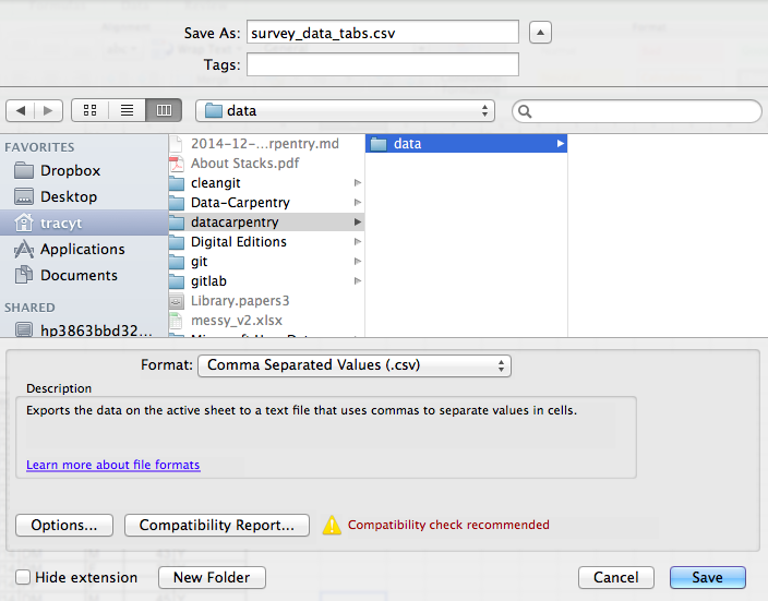
To save a file you have opened in Excel in CSV format:
- From the top menu select ‘File’ and ‘Save as’.
- In the ‘Format’ field, from the list, select ‘Comma Separated
Values’ (
*.csv). - Double check the file name and the location where you want to save it and hit ‘Save’.
An important note for backwards compatibility: you can open CSV files in Excel!
A note on R and xls: There are R
packages that can read xls files (as well as Google
spreadsheets). It is even possible to access different worksheets in the
xls documents.
But
- some of these only work on Windows.
- this equates to replacing a (simple but manual) export to
csvwith additional complexity/dependencies in the data analysis R code. - data formatting best practice still apply.
- Is there really a good reason why
csv(or similar) is not adequate?
Caveats on commas
In some datasets, the data values themselves may include commas (,). In that case, the software which you use (including Excel) will most likely incorrectly display the data in columns. This is because the commas which are a part of the data values will be interpreted as delimiters.
For example, our data might look like this:
species_id,genus,species,taxa
AB,Amphispiza,bilineata,Bird
AH,Ammospermophilus,harrisi,Rodent, not censused
AS,Ammodramus,savannarum,Bird
BA,Baiomys,taylori,Rodent
In the record
AH,Ammospermophilus,harrisi,Rodent, not censused the value
for taxa includes a comma
(Rodent, not censused). If we try to read the above into
Excel (or other spreadsheet program), we will get something like
this:
The value for taxa was split into two columns (instead
of being put in one column D). This can propagate to a
number of further errors. For example, the extra column will be
interpreted as a column with many missing values (and without a proper
header). In addition to that, the value in column D for the
record in row 3 (so the one where the value for ‘taxa’ contained the
comma) is now incorrect.
If you want to store your data in csv format and expect
that your data values may contain commas, you can avoid the problem
discussed above by putting the values in quotes (““). Applying this
rule, our data might look like this:
species_id,genus,species,taxa
"AB","Amphispiza","bilineata","Bird"
"AH","Ammospermophilus","harrisi","Rodent, not censused"
"AS","Ammodramus","savannarum","Bird"
"BA","Baiomys","taylori","Rodent"
Now opening this file as a csv in Excel will not lead to
an extra column, because Excel will only use commas that fall outside of
quotation marks as delimiting characters.
Alternatively, if you are working with data that contains commas, you likely will need to use another delimiter when working in a spreadsheet1. In this case, consider using tabs as your delimiter and working with TSV files. TSV files can be exported from spreadsheet programs in the same way as CSV files.
If you are working with an already existing dataset in which the data values are not included in “” but which have commas as both delimiters and parts of data values, you are potentially facing a major problem with data cleaning. If the dataset you’re dealing with contains hundreds or thousands of records, cleaning them up manually (by either removing commas from the data values or putting the values into quotes - ““) is not only going to take hours and hours but may potentially end up with you accidentally introducing many errors.
Cleaning up datasets is one of the major problems in many scientific disciplines. The approach almost always depends on the particular context. However, it is a good practice to clean the data in an automated fashion, for example by writing and running a script. The Python and R lessons will give you the basis for developing skills to build relevant scripts.
Summary
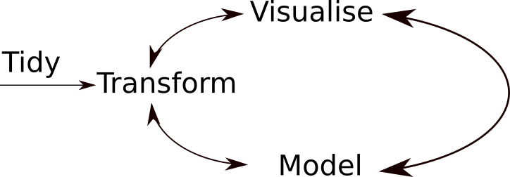
A typical data analysis workflow is illustrated in the figure above, where data is repeatedly transformed, visualised, and modelled. This iteration is repeated multiple times until the data is understood. In many real-life cases, however, most time is spent cleaning up and preparing the data, rather than actually analysing and understanding it.
An agile data analysis workflow, with several fast iterations of the transform/visualise/model cycle is only feasible if the data is formatted in a predictable way and one can reason about the data without having to look at it and/or fix it.
- Good data organization is the foundation of any research project.
This is particularly relevant in European countries where the comma is used as a decimal separator. In such cases, the default value separator in a csv file will be the semi-colon (;), or values will be systematically quoted.↩︎
Content from R and RStudio
Last updated on 2026-07-14 | Edit this page
Overview
Questions
- What are R and RStudio?
Objectives
- Describe the purpose of the RStudio Script, Console, Environment, and Plots panes.
- Organise files and directories for a set of analyses as an R project, and understand the purpose of the working directory.
- Use the built-in RStudio help interface to search for more information on R functions.
- Demonstrate how to provide sufficient information for troubleshooting with the R user community.
This episode is based on the Data Carpentries’s Data Analysis and Visualisation in R for Ecologists lesson.
What is R? What is RStudio?
The term R is used to refer to the programming language, the environment for statistical computing and the software that interprets the scripts written using it.
RStudio is currently a very popular way to not only write your R scripts but also to interact with the R software1. To function correctly, RStudio needs R and therefore both need to be installed on your computer.
The RStudio IDE Cheat Sheet provides much more information than will be covered here, but can be useful to learn keyboard shortcuts and discover new features.
Why learn R?
R does not involve lots of pointing and clicking, and that’s a good thing
The learning curve might be steeper than with other software, but with R, the results of your analysis do not rely on remembering a succession of pointing and clicking, but instead on a series of written commands, and that’s a good thing! So, if you want to redo your analysis because you collected more data, you don’t have to remember which button you clicked in which order to obtain your results; you just have to run your script again.
Working with scripts makes the steps you used in your analysis clear, and the code you write can be inspected by someone else who can give you feedback and spot mistakes.
Working with scripts forces you to have a deeper understanding of what you are doing, and facilitates your learning and comprehension of the methods you use.
R code is great for reproducibility
Reproducibility means that someone else (including your future self) can obtain the same results from the same dataset when using the same analysis code.
R integrates with other tools to generate manuscripts or reports from your code. If you collect more data, or fix a mistake in your dataset, the figures and the statistical tests in your manuscript or report are updated automatically.
An increasing number of journals and funding agencies expect analyses to be reproducible, so knowing R will give you an edge with these requirements.
R is interdisciplinary and extensible
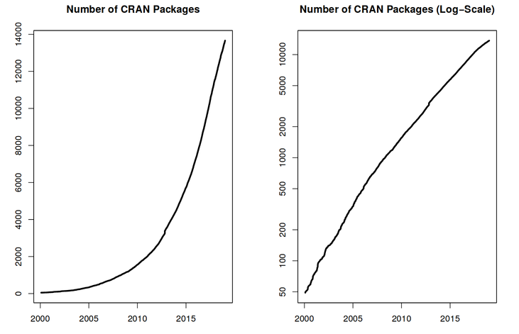
With 10000+ packages2 that can be installed to extend its capabilities, R provides a framework that allows you to combine statistical approaches from many scientific disciplines to best suit the analytical framework you need to analyse your data. For instance, R has packages for image analysis, GIS, time series, population genetics, and a lot more.
R works on data of all shapes and sizes
The skills you learn with R scale easily with the size of your dataset. Whether your dataset has hundreds or millions of lines, it won’t make much difference to you.
R is designed for data analysis. It comes with special data structures and data types that make handling of missing data and statistical factors convenient.
R can connect to spreadsheets, databases, and many other data formats, on your computer or on the web.
R produces high-quality graphics
The plotting functionalities in R are extensive, and allow you to adjust any aspect of your graph to convey most effectively the message from your data.
R has a large and welcoming community
Thousands of people use R daily. Many of them are willing to help you through mailing lists and websites such as Stack Overflow, or on the RStudio community. These broad user communities extend to specialised areas such as bioinformatics. One such subset of the R community is Bioconductor, a scientific project for analysis and comprehension “of data from current and emerging biological assays.” This workshop was developed by members of the Bioconductor community; for more information on Bioconductor, please see the companion workshop “The Bioconductor Project”.
Knowing your way around RStudio
Let’s start by learning about RStudio, which is an Integrated Development Environment (IDE) for working with R.
The RStudio IDE open-source product is free under the Affero General Public License (AGPL) v3. The RStudio IDE is also available with a commercial license and priority email support from Posit, Inc.
We will use the RStudio IDE to write code, navigate the files on our computer, inspect the variables we are going to create, and visualise the plots we will generate. RStudio can also be used for other things (e.g., version control, developing packages, writing Shiny apps) that we will not cover during the workshop.
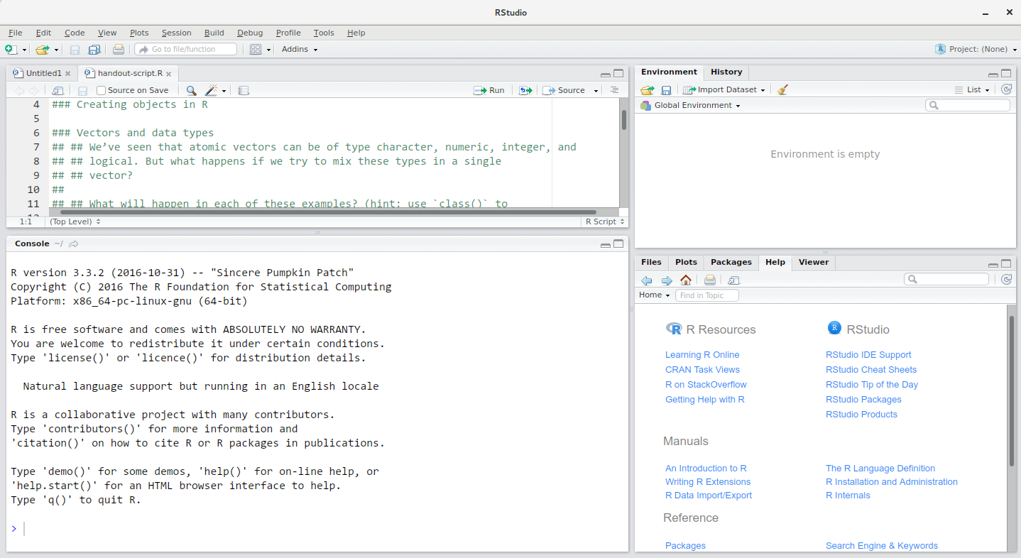
The RStudio window is divided into 4 “Panes”:
- the Source for your scripts and documents (top-left, in the default layout)
- your Environment/History (top-right),
- your Files/Plots/Packages/Help/Viewer (bottom-right), and
- the R Console (bottom-left).
The placement of these panes and their content can be customised (see
menu, Tools -> Global Options -> Pane Layout).
One of the advantages of using RStudio is that all the information you need to write code is available in a single window. Additionally, with many shortcuts, autocompletion, and highlighting for the major file types you use while developing in R, RStudio will make typing easier and less error-prone.
Getting set up
It is good practice to keep a set of related data, analyses, and text self-contained in a single folder, called the working directory. All of the scripts within this folder can then use relative paths to files that indicate where inside the project a file is located (as opposed to absolute paths, which point to where a file is on a specific computer). Working this way makes it a lot easier to move your project around on your computer and share it with others without worrying about whether or not the underlying scripts will still work.
RStudio provides a helpful set of tools to do this through its “Projects” interface, which not only creates a working directory for you, but also remembers its location (allowing you to quickly navigate to it) and optionally preserves custom settings and open files to make it easier to resume work after a break. Go through the steps for creating an “R Project” for this tutorial below.
- Start RStudio.
- Under the
Filemenu, click onNew project. ChooseNew directory, thenNew project. - Enter a name for this new folder (or “directory”), and choose a
convenient location for it. This will be your working
directory for this session (or whole course) (e.g.,
bioc-intro). - Click on
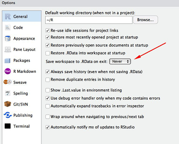
Create project. - (Optional) Set Preferences to ‘Never’ save workspace in RStudio.
RStudio’s default preferences generally work well, but saving a workspace to .RData can be cumbersome, especially if you are working with larger datasets. To turn that off, go to Tools –> ‘Global Options’ and select the ‘Never’ option for ‘Save workspace to .RData’ on exit.
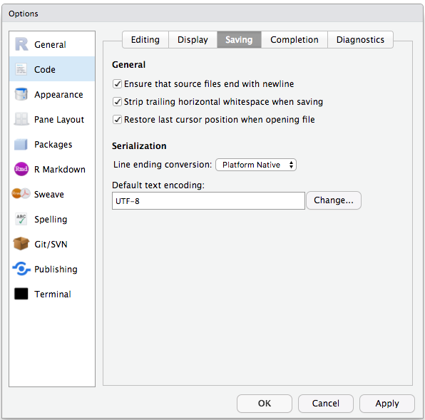
To avoid character encoding issues between Windows and other operating systems, we are going to set UTF-8 by default:
Organizing your working directory
Using a consistent folder structure across your projects will help keep things organised, and will also make it easy to find/file things in the future. This can be especially helpful when you have multiple projects. In general, you may create directories (folders) for scripts, data, and documents.
-
data/Use this folder to store your raw data and intermediate datasets you may create for the need of a particular analysis. For the sake of transparency and provenance, you should always keep a copy of your raw data accessible and do as much of your data cleanup and preprocessing programmatically (i.e., with scripts, rather than manually) as possible. Separating raw data from processed data is also a good idea. For example, you could have filesdata/raw/tree_survey.plot1.txtand...plot2.txtkept separate from adata/processed/tree.survey.csvfile generated by thescripts/01.preprocess.tree_survey.Rscript. -
documents/This would be a place to keep outlines, drafts, and other text. -
scripts/(orsrc) This would be the location to keep your R scripts for different analyses or plotting, and potentially a separate folder for your functions (more on that later).
You may want additional directories or subdirectories depending on your project needs, but these should form the backbone of your working directory.
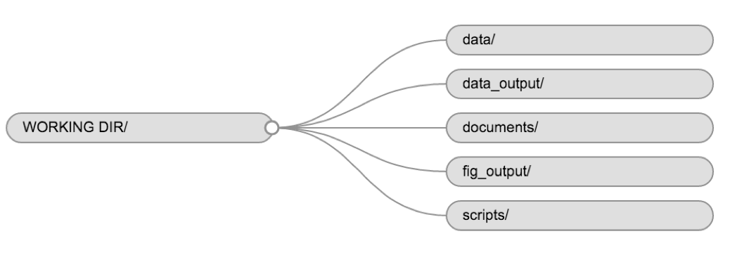
For this course, we will need a data/ folder to store
our raw data, and we will use data_output/ for when we
learn how to export data as CSV files, and fig_output/
folder for the figures that we will save.
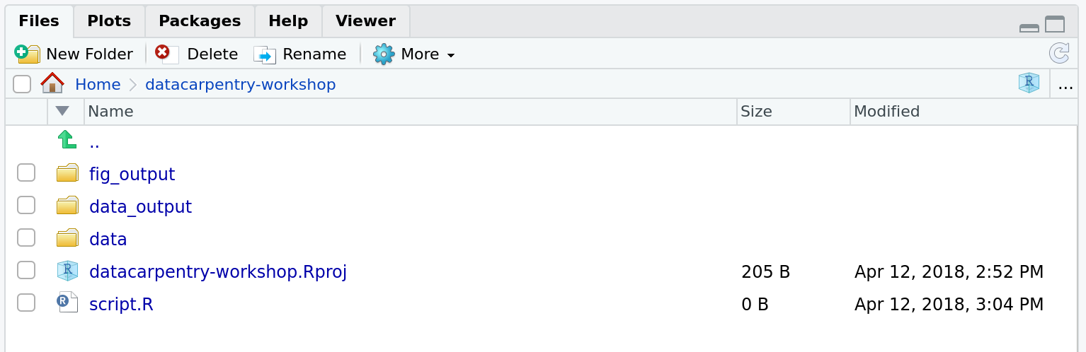
Challenge: create your project directory structure
Under the Files tab on the right of the screen, click on
New Folder and create a folder named data
within your newly created working directory (e.g.,
~/bioc-intro/data). (Alternatively, type
dir.create("data") at your R console.) Repeat these
operations to create a data_output/ and a
fig_output folders.
We are going to keep the script in the root of our working directory because we are only going to use one file and it will make things easier.
Your working directory should now look like this:
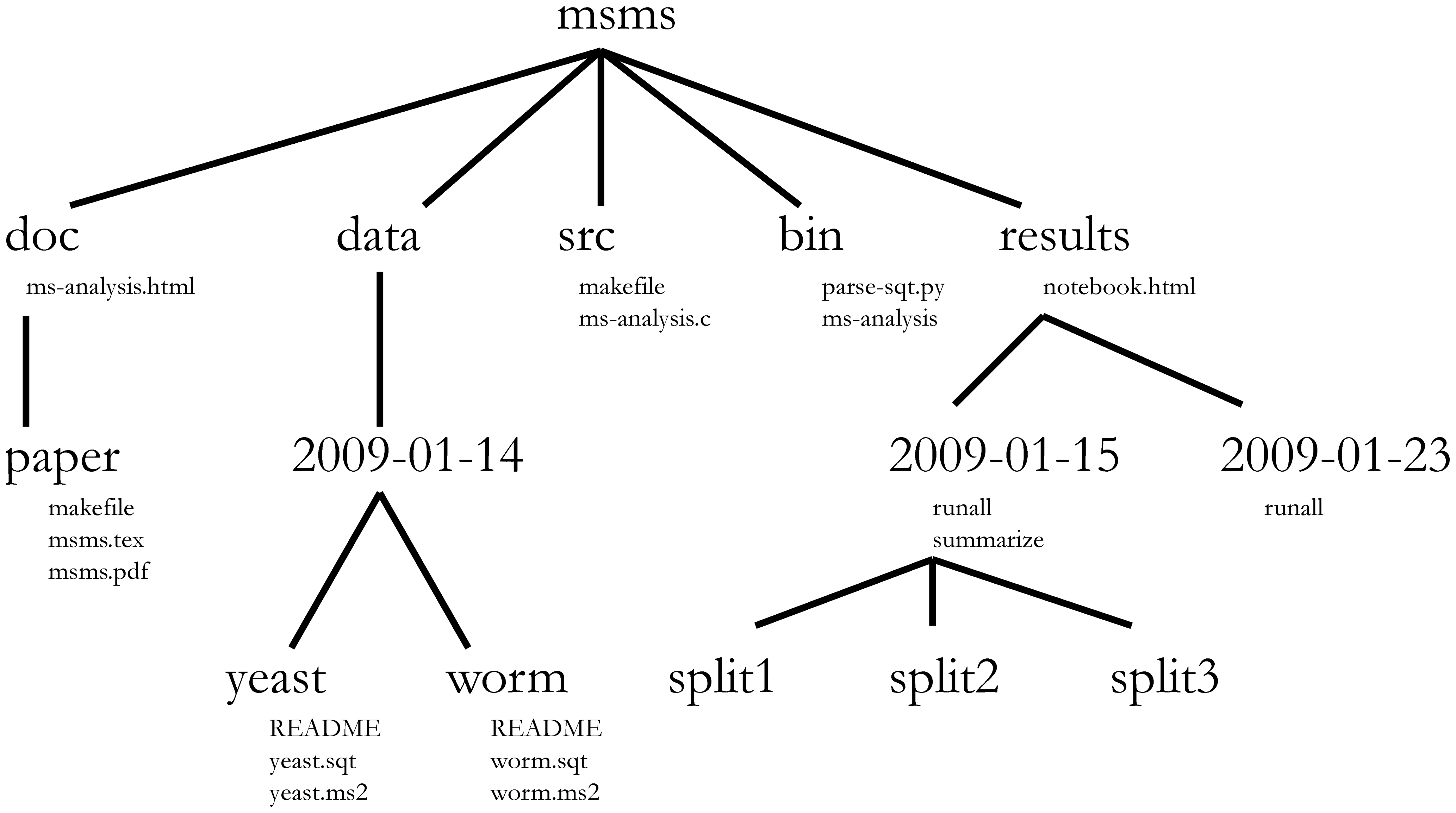
Project management is also applicable to bioinformatics projects, of course3. William Noble (@Noble:2009) proposes the following directory structure:
Directory names are in large typeface, and filenames are in smaller typeface. Only a subset of the files are shown here. Note that the dates are formatted
<year>-<month>-<day>so that they can be sorted in chronological order. The source codesrc/ms-analysis.cis compiled to createbin/ms-analysisand is documented indoc/ms-analysis.html. TheREADMEfiles in the data directories specify who downloaded the data files from what URL on what date. The driver scriptresults/2009-01-15/runallautomatically generates the three subdirectories split1, split2, and split3, corresponding to three cross-validation splits. Thebin/parse-sqt.pyscript is called by both of therunalldriver scripts.
The most important aspect of a well defined and well documented project directory is to enable someone unfamiliar with the project4 to
understand what the project is about, what data are available, what analyses were run, and what results were produced and, most importantly to
repeat the analysis over again - with new data, or changing some analysis parameters.
The working directory
The working directory is an important concept to understand. It is the place from where R will be looking for and saving the files. When you write code for your project, it should refer to files in relation to the root of your working directory and only need files within this structure.
Using RStudio projects makes this easy and ensures that your working
directory is set properly. If you need to check it, you can use
getwd(). If for some reason your working directory is not
what it should be, you can change it in the RStudio interface by
navigating in the file browser where your working directory should be,
and clicking on the blue gear icon More, and select
Set As Working Directory. Alternatively you can use
setwd("/path/to/working/directory") to reset your working
directory. However, your scripts should not include this line because it
will fail on someone else’s computer.
Example
The schema below represents the working directory
bioc-intro with the data and
fig_output sub-directories, and 2 files in the latter:
bioc-intro/data/
          /fig_output/fig1.pdf
          /fig_output/fig2.png
If we were in the working directory, we could refer to the
fig1.pdf file using the relative path
bioc-intro/fig_output/fig1.pdf or the absolute path
/home/user/bioc-intro/fig_output/fig1.pdf.
If we were in the data directory, we would use the
relative path ../fig_output/fig1.pdf or the same absolute
path /home/user/bioc-intro/fig_output/fig1.pdf.
Interacting with R
The basis of programming is that we write down instructions for the computer to follow, and then we tell the computer to follow those instructions. We write, or code, instructions in R because it is a common language that both the computer and we can understand. We call the instructions commands and we tell the computer to follow the instructions by executing (also called running) those commands.
There are two main ways of interacting with R: by using the
console or by using scripts (plain
text files that contain your code). The console pane (in RStudio, the
bottom left panel) is the place where commands written in the R language
can be typed and executed immediately by the computer. It is also where
the results will be shown for commands that have been executed. You can
type commands directly into the console and press Enter to
execute those commands, but they will be forgotten when you close the
session.
Because we want our code and workflow to be reproducible, it is better to type the commands we want in the script editor, and save the script. This way, there is a complete record of what we did, and anyone (including our future selves!) can easily replicate the results on their computer. Note, however, that merely typing the commands in the script does not automatically run them - they still need to be sent to the console for execution.
RStudio allows you to execute commands directly from the script
editor by using the Ctrl + Enter shortcut (on
Macs, Cmd + Return will work, too). The
command on the current line in the script (indicated by the cursor) or
all of the commands in the currently selected text will be sent to the
console and executed when you press Ctrl +
Enter. You can find other keyboard shortcuts in this RStudio
cheatsheet about the RStudio IDE.
At some point in your analysis you may want to check the content of a
variable or the structure of an object, without necessarily keeping a
record of it in your script. You can type these commands and execute
them directly in the console. RStudio provides the Ctrl +
1 and Ctrl + 2 shortcuts allow
you to jump between the script and the console panes.
If R is ready to accept commands, the R console shows a
> prompt. If it receives a command (by typing,
copy-pasting or sending from the script editor using Ctrl +
Enter), R will try to execute it, and when ready, will show
the results and come back with a new > prompt to wait
for new commands.
If R is still waiting for you to enter more data because it isn’t
complete yet, the console will show a + prompt. It means
that you haven’t finished entering a complete command. This is because
you have not ‘closed’ a parenthesis or quotation, i.e. you don’t have
the same number of left-parentheses as right-parentheses, or the same
number of opening and closing quotation marks. When this happens, and
you thought you finished typing your command, click inside the console
window and press Esc; this will cancel the incomplete
command and return you to the > prompt.
How to learn more during and after the course?
The material we cover during this course will give you an initial taste of how you can use R to analyse data for your own research. However, you will need to learn more to do advanced operations such as cleaning your dataset, using statistical methods, or creating beautiful graphics5. The best way to become proficient and efficient at R, as with any other tool, is to use it to address your actual research questions. As a beginner, it can feel daunting to have to write a script from scratch, and given that many people make their code available online, modifying existing code to suit your purpose might make it easier for you to get started.
Seeking help
Use the built-in RStudio help interface to search for more information on R functions
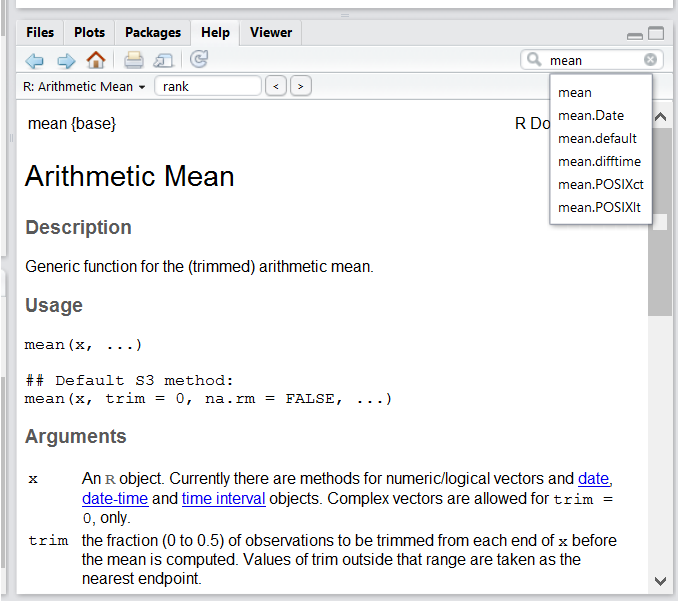
One of the fastest ways to get help, is to use the RStudio help interface. This panel by default can be found at the lower right hand panel of RStudio. As seen in the screenshot, by typing the word “Mean”, RStudio tries to also give a number of suggestions that you might be interested in. The description is then shown in the display window.
I know the name of the function I want to use, but I’m not sure how to use it
If you need help with a specific function, let’s say
barplot(), you can type:
R
?barplot
If you just need to remind yourself of the names of the arguments, you can use:
R
args(lm)
I want to use a function that does X, there must be a function for it but I don’t know which one…
If you are looking for a function to do a particular task, you can
use the help.search() function, which is called by the
double question mark ??. However, this only looks through
the installed packages for help pages with a match to your search
request
R
??kruskal
If you can’t find what you are looking for, you can use the rdocumentation.org website that searches through the help files across all packages available.
Finally, a generic Google or internet search “R <task>” will often either send you to the appropriate package documentation or a helpful forum where someone else has already asked your question.
I am stuck… I get an error message that I don’t understand
Start by googling the error message. However, this doesn’t always work very well because often, package developers rely on the error catching provided by R. You end up with general error messages that might not be very helpful to diagnose a problem (e.g. “subscript out of bounds”). If the message is very generic, you might also include the name of the function or package you’re using in your query.
However, you should check Stack Overflow. Search using the
[r] tag. Most questions have already been answered, but the
challenge is to use the right words in the search to find the
answers:
https://stackoverflow.com/questions/tagged/r
The Introduction to R can also be dense for people with little programming experience but it is a good place to understand the underpinnings of the R language.
The R FAQ is dense and technical but it is full of useful information.
Asking for help
The key to receiving help from someone is for them to rapidly grasp your problem. You should make it as easy as possible to pinpoint where the issue might be.
Try to use the correct words to describe your problem. For instance, a package is not the same thing as a library. Most people will understand what you meant, but others have really strong feelings about the difference in meaning. The key point is that it can make things confusing for people trying to help you. Be as precise as possible when describing your problem.
If possible, try to reduce what doesn’t work to a simple reproducible example. If you can reproduce the problem using a very small data frame instead of your 50000 rows and 10000 columns one, provide the small one with the description of your problem. When appropriate, try to generalise what you are doing so even people who are not in your field can understand the question. For instance instead of using a subset of your real dataset, create a small (3 columns, 5 rows) generic one. For more information on how to write a reproducible example see this article by Hadley Wickham.
To share an object with someone else, if it’s relatively small, you
can use the function dput(). It will output R code that can
be used to recreate the exact same object as the one in memory:
R
## iris is an example data frame that comes with R and head() is a
## function that returns the first part of the data frame
dput(head(iris))
OUTPUT
structure(list(Sepal.Length = c(5.1, 4.9, 4.7, 4.6, 5, 5.4),
    Sepal.Width = c(3.5, 3, 3.2, 3.1, 3.6, 3.9), Petal.Length = c(1.4,
    1.4, 1.3, 1.5, 1.4, 1.7), Petal.Width = c(0.2, 0.2, 0.2,
    0.2, 0.2, 0.4), Species = structure(c(1L, 1L, 1L, 1L, 1L,
    1L), levels = c("setosa", "versicolor", "virginica"), class = "factor")), row.names = c(NA,
6L), class = "data.frame")
If the object is larger, provide either the raw file (i.e., your CSV file) with your script up to the point of the error (and after removing everything that is not relevant to your issue). Alternatively, in particular if your question is not related to a data frame, you can save any R object to a file[^export]:
R
saveRDS(iris, file="/tmp/iris.rds")
The content of this file is however not human readable and cannot be
posted directly on Stack Overflow. Instead, it can be sent to someone by
email who can read it with the readRDS() command (here it
is assumed that the downloaded file is in a Downloads
folder in the user’s home directory):
R
some_data <- readRDS(file="~/Downloads/iris.rds")
Last, but certainly not least, always include the output of
sessionInfo() as it provides critical information
about your platform, the versions of R and the packages that you are
using, and other information that can be very helpful to understand your
problem.
R
sessionInfo()
OUTPUT
R version 4.6.0 (2026-04-24)
Platform: x86_64-pc-linux-gnu
Running under: Ubuntu 24.04.4 LTS

Matrix products: default
BLAS:   /usr/lib/x86_64-linux-gnu/openblas-pthread/libblas.so.3
LAPACK: /usr/lib/x86_64-linux-gnu/openblas-pthread/libopenblasp-r0.3.26.so;  LAPACK version 3.12.0

locale:
 [1] LC_CTYPE=en_US.UTF-8       LC_NUMERIC=C
 [3] LC_TIME=en_US.UTF-8        LC_COLLATE=en_US.UTF-8
 [5] LC_MONETARY=en_US.UTF-8    LC_MESSAGES=en_US.UTF-8
 [7] LC_PAPER=en_US.UTF-8       LC_NAME=C
 [9] LC_ADDRESS=C               LC_TELEPHONE=C
[11] LC_MEASUREMENT=en_US.UTF-8 LC_IDENTIFICATION=C

time zone: Etc/UTC
tzcode source: system (glibc)

attached base packages:
[1] stats     graphics  grDevices utils     datasets  methods   base

loaded via a namespace (and not attached):
 [1] BiocManager_1.30.27 compiler_4.6.0      cli_3.6.6
 [4] tools_4.6.0         otel_0.2.0          yaml_2.3.12
 [7] knitr_1.51          xfun_0.60           rlang_1.3.0
[10] renv_1.2.3          evaluate_1.0.5
Where to ask for help?
- The person sitting next to you during the course. Don’t hesitate to talk to your neighbour during the workshop, compare your answers, and ask for help.
- Your friendly colleagues: if you know someone with more experience than you, they might be able and willing to help you.
- Stack Overflow: if your question hasn’t been answered before and is well crafted, chances are you will get an answer in less than 5 min. Remember to follow their guidelines on how to ask a good question.
- The R-help mailing list: it is read by a lot of people (including most of the R core team), a lot of people post to it, but the tone can be pretty dry, and it is not always very welcoming to new users. If your question is valid, you are likely to get an answer very fast but don’t expect that it will come with smiley faces. Also, here more than anywhere else, be sure to use correct vocabulary (otherwise you might get an answer pointing to the misuse of your words rather than answering your question). You will also have more success if your question is about a base function rather than a specific package.
- If your question is about a specific package, see if there is a
mailing list for it. Usually it’s included in the DESCRIPTION file of
the package that can be accessed using
packageDescription("name-of-package"). You may also want to try to email the author of the package directly, or open an issue on the code repository (e.g., GitHub). - There are also some topic-specific mailing lists (GIS, phylogenetics, etc…), the complete list is available on the R-project mailing list page.
More resources
The Posting Guide for the R mailing lists.
How to ask for R help useful guidelines.
This blog post by Jon Skeet has quite comprehensive advice on how to ask programming questions.
The reprex package is very helpful to create reproducible examples when asking for help. The rOpenSci community call “How to ask questions so they get answered” (Github link and video recording) includes a presentation of the reprex package and of its philosophy.
R packages
Loading packages
As we have seen above, R packages play a fundamental role in R. The
make use of a package’s functionality, assuming it is installed, we
first need to load it to be able to use it. This is done with the
library() function. Below, we load
ggplot2.
R
library("ggplot2")
Installing packages
The default package repository is The Comprehensive R Archive
Network (CRAN), and any package that is available on CRAN can be
installed with the install.packages() function. Below, for
example, we install the dplyr package that we will learn
about later.
R
install.packages("dplyr")
This command will install the dplyr package as well as
all its dependencies, i.e. all the packages that it relies on to
function.
Another major R package repository is maintained by Bioconductor. Bioconductor
packages are managed and installed using a dedicated package, namely
BiocManager, that can be installed from CRAN with
R
install.packages("BiocManager")
Individual packages such as SummarizedExperiment (we
will use it later), DESeq2 (for RNA-Seq analysis), and any
others from either Bioconductor or CRAN can then be installed with
BiocManager::install.
R
BiocManager::install("SummarizedExperiment")
BiocManager::install("DESeq2")
By default, BiocManager::install() will also check all
your installed packages and see if there are newer versions available.
If there are, it will show them to you and ask you if you want to
Update all/some/none? [a/s/n]: and then wait for your
answer. While you should strive to have the most up-to-date package
versions, in practice we recommend only updating packages in a fresh R
session before any packages are loaded.
- Start using R and RStudio
As opposed to using R directly from the command line console. There exist other software that interface and integrate with R, but RStudio is particularly well suited for beginners while providing numerous very advanced features.↩︎
i.e. add-ons that confer R with new functionality, such as bioinformatics data analysis.↩︎
In this course, we consider bioinformatics as data science applied to biological or bio-medical data.↩︎
That someone could be, and very likely will be your future self, a couple of months or years after the analyses were run.↩︎
We will introduce most of these (except statistics) here, but will only manage to scratch the surface of the wealth of what is possible to do with R.↩︎
Content from Introduction to R
Last updated on 2026-07-14 | Edit this page
Overview
Questions
- First commands in R
Objectives
- Define the following terms as they relate to R: object, assign, call, function, arguments, options.
- Assign values to objects in R.
- Learn how to name objects
- Use comments to inform script.
- Solve simple arithmetic operations in R.
- Call functions and use arguments to change their default options.
- Inspect the content of vectors and manipulate their content.
- Subset and extract values from vectors.
- Analyze vectors with missing data.
This episode is based on the Data Carpentries’s Data Analysis and Visualisation in R for Ecologists lesson.
Creating objects in R
You can get output from R simply by typing math in the console:
R
3 + 5
OUTPUT
[1] 8R
12 / 7
OUTPUT
[1] 1.714286However, to do useful and interesting things, we need to assign
values to objects. To create an object, we need to
give it a name followed by the assignment operator <-,
and the value we want to give it:
R
weight_kg <- 55
<- is the assignment operator. It assigns values on
the right to objects on the left. So, after executing
x <- 3, the value of x is 3.
The arrow can be read as 3 goes into x.
For historical reasons, you can also use = for assignments,
but not in every context. Because of the slight
differences in syntax, it is good practice to always use
<- for assignments.
In RStudio, typing Alt + - (push Alt
at the same time as the - key) will write <-
in a single keystroke in a PC, while typing Option +
- (push Option at the same time as the
- key) does the same in a Mac.
Naming variables
Objects can be given any name such as x,
current_temperature, or subject_id. You want
your object names to be explicit and not too long. They cannot start
with a number (2x is not valid, but x2 is). R
is case sensitive (e.g., weight_kg is different from
Weight_kg). There are some names that cannot be used
because they are the names of fundamental functions in R (e.g.,
if, else, for, see the Reserved
Words in R manual page, for a complete list). In general, even if
it’s allowed, it’s best to not use other function names (e.g.,
c, T, mean, data,
df, weights). If in doubt, check the help to
see if the name is already in use. It’s also best to avoid dots
(.) within an object name as in my.dataset.
There are many functions in R with dots in their names for historical
reasons, but because dots have a special meaning in R (for methods) and
other programming languages, it’s best to avoid them. It is also
recommended to use nouns for object names, and verbs for function names.
It’s important to be consistent in the styling of your code (where you
put spaces, how you name objects, etc.). Using a consistent coding style
makes your code clearer to read for your future self and your
collaborators. In R, some popular style guides are Google’s, the
tidyverse’s style and the Bioconductor
style guide. The tidyverse’s is very comprehensive and may seem
overwhelming at first. You can install the lintr
package to automatically check for issues in the styling of your
code.
Objects vs. variables: What are known as
objectsinRare known asvariablesin many other programming languages. Depending on the context,objectandvariablecan have drastically different meanings. However, in this lesson, the two words are used synonymously. For more information see here.
When assigning a value to an object, R does not print anything. You can force R to print the value by using parentheses or by typing the object name:
R
weight_kg <- 55    # doesn't print anything
(weight_kg <- 55)  # but putting parenthesis around the call prints the value of `weight_kg`
OUTPUT
[1] 55R
weight_kg # and so does typing the name of the object
OUTPUT
[1] 55Now that R has weight_kg in memory, we can do arithmetic
with it. For instance, we may want to convert this weight into pounds
(weight in pounds is 2.2 times the weight in kg):
R
2.2 * weight_kg
OUTPUT
[1] 121We can also change an object’s value by assigning it a new one:
R
weight_kg <- 57.5
2.2 * weight_kg
OUTPUT
[1] 126.5This means that assigning a value to one object does not change the
values of other objects For example, let’s store the animal’s weight in
pounds in a new object, weight_lb:
R
weight_lb <- 2.2 * weight_kg
and then change weight_kg to 100.
R
weight_kg <- 100
Challenge:
What do you think is the current content of the object
weight_lb? 126.5 or 220?
Comments
The comment character in R is #, anything to the right
of a # in a script will be ignored by R. It is useful to
leave notes, and explanations in your scripts.
RStudio makes it easy to comment or uncomment a paragraph: after selecting the lines you want to comment, press at the same time on your keyboard Ctrl + Shift + C. If you only want to comment out one line, you can put the cursor at any location of that line (i.e. no need to select the whole line), then press Ctrl + Shift + C.
Challenge
What are the values after each statement in the following?
R
mass <- 47.5            # mass?
age  <- 122             # age?
mass <- mass * 2.0      # mass?
age  <- age - 20        # age?
mass_index <- mass/age  # mass_index?
Functions and their arguments
Functions are “canned scripts” that automate more complicated sets of
commands including operations assignments, etc. Many functions are
predefined, or can be made available by importing R packages
(more on that later). A function usually gets one or more inputs called
arguments. Functions often (but not always) return a
value. A typical example would be the function
sqrt(). The input (the argument) must be a number, and the
return value (in fact, the output) is the square root of that number.
Executing a function (‘running it’) is called calling the
function. An example of a function call is:
R
b <- sqrt(a)
Here, the value of a is given to the sqrt()
function, the sqrt() function calculates the square root,
and returns the value which is then assigned to the object
b. This function is very simple, because it takes just one
argument.
The return ‘value’ of a function need not be numerical (like that of
sqrt()), and it also does not need to be a single item: it
can be a set of things, or even a dataset. We’ll see that when we read
data files into R.
Arguments can be anything, not only numbers or filenames, but also other objects. Exactly what each argument means differs per function, and must be looked up in the documentation (see below). Some functions take arguments which may either be specified by the user, or, if left out, take on a default value: these are called options. Options are typically used to alter the way the function operates, such as whether it ignores ‘bad values’, or what symbol to use in a plot. However, if you want something specific, you can specify a value of your choice which will be used instead of the default.
Let’s try a function that can take multiple arguments:
round().
R
round(3.14159)
OUTPUT
[1] 3Here, we’ve called round() with just one argument,
3.14159, and it has returned the value 3.
That’s because the default is to round to the nearest whole number. If
we want more digits we can see how to do that by getting information
about the round function. We can use
args(round) or look at the help for this function using
?round.
R
args(round)
OUTPUT
function (x, digits = 0, ...)
NULL
R
?round
We see that if we want a different number of digits, we can type
digits=2 or however many we want.
R
round(3.14159, digits = 2)
OUTPUT
[1] 3.14If you provide the arguments in the exact same order as they are defined you don’t have to name them:
R
round(3.14159, 2)
OUTPUT
[1] 3.14And if you do name the arguments, you can switch their order:
R
round(digits = 2, x = 3.14159)
OUTPUT
[1] 3.14It’s good practice to put the non-optional arguments (like the number you’re rounding) first in your function call, and to specify the names of all optional arguments. If you don’t, someone reading your code might have to look up the definition of a function with unfamiliar arguments to understand what you’re doing. By specifying the name of the arguments you are also safeguarding against possible future changes in the function interface, which may potentially add new arguments in between the existing ones.
Vectors and data types
A vector is the most common and basic data type in R, and is pretty
much the workhorse of R. A vector is composed by a series of values,
such as numbers or characters. We can assign a series of values to a
vector using the c() function. For example we can create a
vector of animal weights and assign it to a new object
weight_g:
R
weight_g <- c(50, 60, 65, 82)
weight_g
OUTPUT
[1] 50 60 65 82A vector can also contain characters:
R
molecules <- c("dna", "rna", "protein")
molecules
OUTPUT
[1] "dna" "rna" "protein"The quotes around “dna”, “rna”, etc. are essential here. Without the
quotes R will assume there are objects called dna,
rna and protein. As these objects don’t exist
in R’s memory, there will be an error message.
There are many functions that allow you to inspect the content of a
vector. length() tells you how many elements are in a
particular vector:
R
length(weight_g)
OUTPUT
[1] 4R
length(molecules)
OUTPUT
[1] 3An important feature of a vector, is that all of the elements are the
same type of data. The function class() indicates the class
(the type of element) of an object:
R
class(weight_g)
OUTPUT
[1] "numeric"R
class(molecules)
OUTPUT
[1] "character"The function str() provides an overview of the structure
of an object and its elements. It is a useful function when working with
large and complex objects:
R
str(weight_g)
OUTPUT
num [1:4] 50 60 65 82R
str(molecules)
OUTPUT
chr [1:3] "dna" "rna" "protein"You can use the c() function to add other elements to
your vector:
R
weight_g <- c(weight_g, 90) # add to the end of the vector
weight_g <- c(30, weight_g) # add to the beginning of the vector
weight_g
OUTPUT
[1] 30 50 60 65 82 90In the first line, we take the original vector weight_g,
add the value 90 to the end of it, and save the result back
into weight_g. Then we add the value 30 to the
beginning, again saving the result back into weight_g.
We can do this over and over again to grow a vector, or assemble a dataset. As we program, this may be useful to add results that we are collecting or calculating.
An atomic vector is the simplest R data
type and is a linear vector of a single type. Above, we saw 2
of the 6 main atomic vector types that R uses:
"character" and "numeric" (or
"double"). These are the basic building blocks that all R
objects are built from. The other 4 atomic vector types
are:
-
"logical"forTRUEandFALSE(the boolean data type) -
"integer"for integer numbers (e.g.,2L, theLindicates to R that it’s an integer) -
"complex"to represent complex numbers with real and imaginary parts (e.g.,1 + 4i) and that’s all we’re going to say about them -
"raw"for bitstreams that we won’t discuss further
You can check the type of your vector using the typeof()
function and inputting your vector as the argument.
Vectors are one of the many data structures that R
uses. Other important ones are lists (list), matrices
(matrix), data frames (data.frame), factors
(factor) and arrays (array).
Challenge:
We’ve seen that atomic vectors can be of type character, numeric (or double), integer, and logical. But what happens if we try to mix these types in a single vector?
R implicitly converts them to all be the same type
Challenge:
What will happen in each of these examples? (hint: use
class() to check the data type of your objects and type in
their names to see what happens):
R
num_char <- c(1, 2, 3, "a")
num_logical <- c(1, 2, 3, TRUE, FALSE)
char_logical <- c("a", "b", "c", TRUE)
tricky <- c(1, 2, 3, "4")
R
class(num_char)
OUTPUT
[1] "character"R
num_char
OUTPUT
[1] "1" "2" "3" "a"R
class(num_logical)
OUTPUT
[1] "numeric"R
num_logical
OUTPUT
[1] 1 2 3 1 0R
class(char_logical)
OUTPUT
[1] "character"R
char_logical
OUTPUT
[1] "a" "b" "c" "TRUE"R
class(tricky)
OUTPUT
[1] "character"R
tricky
OUTPUT
[1] "1" "2" "3" "4"Challenge:
Why do you think it happens?
Vectors can be of only one data type. R tries to convert (coerce) the content of this vector to find a common denominator that doesn’t lose any information.
Challenge:
How many values in combined_logical are
"TRUE" (as a character) in the following example:
R
num_logical <- c(1, 2, 3, TRUE)
char_logical <- c("a", "b", "c", TRUE)
combined_logical <- c(num_logical, char_logical)
Only one. There is no memory of past data types, and the coercion
happens the first time the vector is evaluated. Therefore, the
TRUE in num_logical gets converted into a
1 before it gets converted into "1" in
combined_logical.
R
combined_logical
OUTPUT
[1] "1" "2" "3" "1" "a" "b" "c" "TRUE"Challenge:
In R, we call converting objects from one class into another class coercion. These conversions happen according to a hierarchy, whereby some types get preferentially coerced into other types. Can you draw a diagram that represents the hierarchy of how these data types are coerced?
logical → numeric → character ← logical
Subsetting vectors
If we want to extract one or several values from a vector, we must provide one or several indices in square brackets. For instance:
R
molecules <- c("dna", "rna", "peptide", "protein")
molecules[2]
OUTPUT
[1] "rna"R
molecules[c(3, 2)]
OUTPUT
[1] "peptide" "rna" We can also repeat the indices to create an object with more elements than the original one:
R
more_molecules <- molecules[c(1, 2, 3, 2, 1, 4)]
more_molecules
OUTPUT
[1] "dna" "rna" "peptide" "rna" "dna" "protein"R indices start at 1. Programming languages like Fortran, MATLAB, Julia, and R start counting at 1, because that’s what human beings typically do. Languages in the C family (including C++, Java, Perl, and Python) count from 0 because that’s simpler for computers to do.
Finally, it is also possible to get all the elements of a vector except some specified elements using negative indices:
R
molecules ## all molecules
OUTPUT
[1] "dna" "rna" "peptide" "protein"R
molecules[-1] ## all but the first one
OUTPUT
[1] "rna" "peptide" "protein"R
molecules[-c(1, 3)] ## all but 1st/3rd ones
OUTPUT
[1] "rna" "protein"R
molecules[c(-1, -3)] ## all but 1st/3rd ones
OUTPUT
[1] "rna" "protein"Conditional subsetting
Another common way of subsetting is by using a logical vector.
TRUE will select the element with the same index, while
FALSE will not:
R
weight_g <- c(21, 34, 39, 54, 55)
weight_g[c(TRUE, FALSE, TRUE, TRUE, FALSE)]
OUTPUT
[1] 21 39 54Typically, these logical vectors are not typed by hand, but are the output of other functions or logical tests. For instance, if you wanted to select only the values above 50:
R
## will return logicals with TRUE for the indices that meet
## the condition
weight_g > 50
OUTPUT
[1] FALSE FALSE FALSE TRUE TRUER
## so we can use this to select only the values above 50
weight_g[weight_g > 50]
OUTPUT
[1] 54 55You can combine multiple tests using & (both
conditions are true, AND) or | (at least one of the
conditions is true, OR):
R
weight_g[weight_g < 30 | weight_g > 50]
OUTPUT
[1] 21 54 55R
weight_g[weight_g >= 30 & weight_g == 21]
OUTPUT
numeric(0)Here, < stands for “less than”, > for
“greater than”, >= for “greater than or equal to”, and
== for “equal to”. The double equal sign == is
a test for numerical equality between the left and right hand sides, and
should not be confused with the single = sign, which
performs variable assignment (similar to <-).
A common task is to search for certain strings in a vector. One could
use the “or” operator | to test for equality to multiple
values, but this can quickly become tedious. The function
%in% allows you to test if any of the elements of a search
vector are found:
R
molecules <- c("dna", "rna", "protein", "peptide")
molecules[molecules == "rna" | molecules == "dna"] # returns both rna and dna
OUTPUT
[1] "dna" "rna"R
molecules %in% c("rna", "dna", "metabolite", "peptide", "glycerol")
OUTPUT
[1] TRUE TRUE FALSE TRUER
molecules[molecules %in% c("rna", "dna", "metabolite", "peptide", "glycerol")]
OUTPUT
[1] "dna" "rna" "peptide"Challenge:
Can you figure out why "four" > "five" returns
TRUE?
R
"four" > "five"
OUTPUT
[1] TRUEWhen using > or < on strings, R
compares their alphabetical order. Here "four" comes after
"five", and therefore is greater than it.
Names
It is possible to name each element of a vector. The code chunk below shows an initial vector without any names, how names are set, and retrieved.
R
x <- c(1, 5, 3, 5, 10)
names(x) ## no names
OUTPUT
NULLR
names(x) <- c("A", "B", "C", "D", "E")
names(x) ## now we have names
OUTPUT
[1] "A" "B" "C" "D" "E"When a vector has names, it is possible to access elements by their name, in addition to their index.
R
x[c(1, 3)]
OUTPUT
A C
1 3
R
x[c("A", "C")]
OUTPUT
A C
1 3
Missing data
As R was designed to analyze datasets, it includes the concept of
missing data (which is uncommon in other programming languages). Missing
data are represented in vectors as NA.
When doing operations on numbers, most functions will return
NA if the data you are working with include missing values.
This feature makes it harder to overlook the cases where you are dealing
with missing data. You can add the argument na.rm = TRUE to
calculate the result while ignoring the missing values.
R
heights <- c(2, 4, 4, NA, 6)
mean(heights)
OUTPUT
[1] NAR
max(heights)
OUTPUT
[1] NAR
mean(heights, na.rm = TRUE)
OUTPUT
[1] 4R
max(heights, na.rm = TRUE)
OUTPUT
[1] 6If your data include missing values, you may want to become familiar
with the functions is.na(), na.omit(), and
complete.cases(). See below for examples.
R
## Extract those elements which are not missing values.
heights[!is.na(heights)]
OUTPUT
[1] 2 4 4 6R
## Returns the object with incomplete cases removed.
## The returned object is an atomic vector of type `"numeric"`
## (or `"double"`).
na.omit(heights)
OUTPUT
[1] 2 4 4 6
attr(,"na.action")
[1] 4
attr(,"class")
[1] "omit"
R
## Extract those elements which are complete cases.
## The returned object is an atomic vector of type `"numeric"`
## (or `"double"`).
heights[complete.cases(heights)]
OUTPUT
[1] 2 4 4 6Challenge:
- Using this vector of heights in inches, create a new vector with the NAs removed.
R
heights <- c(63, 69, 60, 65, NA, 68, 61, 70, 61, 59, 64, 69, 63, 63, NA, 72, 65, 64, 70, 63, 65)
- Use the function
median()to calculate the median of theheightsvector. - Use R to figure out how many people in the set are taller than 67 inches.
R
heights_no_na <- heights[!is.na(heights)]
## or
heights_no_na <- na.omit(heights)
R
median(heights, na.rm = TRUE)
OUTPUT
[1] 64R
heights_above_67 <- heights_no_na[heights_no_na > 67]
length(heights_above_67)
OUTPUT
[1] 6Generating vectors
Constructors
There exists some functions to generate vectors of different type. To
generate a vector of numerics, one can use the numeric()
constructor, providing the length of the output vector as parameter. The
values will be initialised with 0.
R
numeric(3)
OUTPUT
[1] 0 0 0R
numeric(10)
OUTPUT
[1] 0 0 0 0 0 0 0 0 0 0Note that if we ask for a vector of numerics of length 0, we obtain exactly that:
R
numeric(0)
OUTPUT
numeric(0)There are similar constructors for characters and logicals, named
character() and logical() respectively.
Challenge:
What are the defaults for character and logical vectors?
R
character(2) ## the empty character
OUTPUT
[1] "" ""R
logical(2) ## FALSE
OUTPUT
[1] FALSE FALSEReplicate elements
The rep function allow to repeat a value a certain
number of times. If we want to initiate a vector of numerics of length 5
with the value -1, for example, we could do the following:
R
rep(-1, 5)
OUTPUT
[1] -1 -1 -1 -1 -1Similarly, to generate a vector populated with missing values, which is often a good way to start, without setting assumptions on the data to be collected:
R
rep(NA, 5)
OUTPUT
[1] NA NA NA NA NArep can take vectors of any length as input (above, we
used vectors of length 1) and any type. For example, if we want to
repeat the values 1, 2 and 3 five times, we would do the following:
R
rep(c(1, 2, 3), 5)
OUTPUT
[1] 1 2 3 1 2 3 1 2 3 1 2 3 1 2 3Challenge:
What if we wanted to repeat the values 1, 2 and 3 five times, but
obtain five 1s, five 2s and five 3s in that order? There are two
possibilities - see ?rep or ?sort for
help.
R
rep(c(1, 2, 3), each = 5)
OUTPUT
[1] 1 1 1 1 1 2 2 2 2 2 3 3 3 3 3R
sort(rep(c(1, 2, 3), 5))
OUTPUT
[1] 1 1 1 1 1 2 2 2 2 2 3 3 3 3 3Sequence generation
Another very useful function is seq, to generate a
sequence of numbers. For example, to generate a sequence of integers
from 1 to 20 by steps of 2, one would use:
R
seq(from = 1, to = 20, by = 2)
OUTPUT
[1] 1 3 5 7 9 11 13 15 17 19The default value of by is 1 and, given that the
generation of a sequence of one value to another with steps of 1 is
frequently used, there’s a shortcut:
R
seq(1, 5, 1)
OUTPUT
[1] 1 2 3 4 5R
seq(1, 5) ## default by
OUTPUT
[1] 1 2 3 4 5R
1:5
OUTPUT
[1] 1 2 3 4 5To generate a sequence of numbers from 1 to 20 of final length of 3, one would use:
R
seq(from = 1, to = 20, length.out = 3)
OUTPUT
[1] 1.0 10.5 20.0Random samples and permutations
A last group of useful functions are those that generate random data.
The first one, sample, generates a random permutation of
another vector. For example, to draw a random order to 10 students oral
exam, I first assign each student a number from 1 to ten (for instance
based on the alphabetic order of their name) and then:
R
sample(1:10)
OUTPUT
[1] 9 4 7 1 2 5 3 10 6 8Without further arguments, sample will return a
permutation of all elements of the vector. If I want a random sample of
a certain size, I would set this value as the second argument. Below, I
sample 5 random letters from the alphabet contained in the pre-defined
letters vector:
R
sample(letters, 5)
OUTPUT
[1] "s" "a" "u" "x" "j"If I wanted an output larger than the input vector, or being able to
draw some elements multiple times, I would need to set the
replace argument to TRUE:
R
sample(1:5, 10, replace = TRUE)
OUTPUT
[1] 2 1 5 5 1 1 5 5 2 2Challenge:
When trying the functions above out, you will have realised that the
samples are indeed random and that one doesn’t get the same permutation
twice. To be able to reproduce these random draws, one can set the
random number generation seed manually with set.seed()
before drawing the random sample.
Test this feature with your neighbour. First draw two random
permutations of 1:10 independently and observe that you get
different results.
Now set the seed with, for example, set.seed(123) and
repeat the random draw. Observe that you now get the same random
draws.
Repeat by setting a different seed.
Different permutations
R
sample(1:10)
OUTPUT
[1] 9 1 4 3 6 2 5 8 10 7R
sample(1:10)
OUTPUT
[1] 4 9 7 6 1 10 8 3 2 5Same permutations with seed 123
R
set.seed(123)
sample(1:10)
OUTPUT
[1] 3 10 2 8 6 9 1 7 5 4R
set.seed(123)
sample(1:10)
OUTPUT
[1] 3 10 2 8 6 9 1 7 5 4A different seed
R
set.seed(1)
sample(1:10)
OUTPUT
[1] 9 4 7 1 2 5 3 10 6 8R
set.seed(1)
sample(1:10)
OUTPUT
[1] 9 4 7 1 2 5 3 10 6 8Drawing samples from a normal distribution
The last function we are going to see is rnorm, that
draws a random sample from a normal distribution. Two normal
distributions of means 0 and 100 and standard deviations 1 and 5, noted
N(0, 1) and N(100, 5), are shown below.
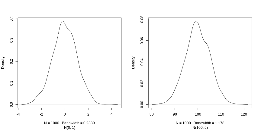
The three arguments, n, mean and
sd, define the size of the sample, and the parameters of
the normal distribution, i.e the mean and its standard deviation. The
defaults of the latter are 0 and 1.
R
rnorm(5)
OUTPUT
[1] 0.69641761 0.05351568 -1.31028350 -2.12306606 -0.20807859R
rnorm(5, 2, 2)
OUTPUT
[1] 1.3744268 -0.1164714 2.8344472 1.3690969 3.6510983R
rnorm(5, 100, 5)
OUTPUT
[1] 106.45636 96.87448 95.62427 100.71678 107.12595Now that we have learned how to write scripts, and the basics of R’s data structures, we are ready to start working with larger data, and learn about data frames.
- How to interact with R
Content from Starting with data
Last updated on 2026-07-14 | Edit this page
Overview
Questions
- First data analysis in R
Objectives
- Describe what a
data.frameis. - Load external data from a .csv file into a data frame.
- Summarize the contents of a data frame.
- Describe what a factor is.
- Convert between strings and factors.
- Reorder and rename factors.
- Format dates.
- Export and save data.
This episode is based on the Data Carpentries’s Data Analysis and Visualisation in R for Ecologists lesson.
Presentation of the gene expression data
We are going to use part of the data published by Blackmore et al. (2017), The effect of upper-respiratory infection on transcriptomic changes in the CNS. The goal of the study was to determine the effect of an upper-respiratory infection on changes in RNA transcription occurring in the cerebellum and spinal cord post infection. Gender matched eight week old C57BL/6 mice were inoculated with saline or with Influenza A by intranasal route and transcriptomic changes in the cerebellum and spinal cord tissues were evaluated by RNA-seq at days 0 (non-infected), 4 and 8.
The dataset is stored as a comma-separated values (CSV) file. Each row holds information for a single RNA expression measurement, and the first eleven columns represent:
| Column | Description |
|---|---|
| gene | The name of the gene that was measured |
| sample | The name of the sample the gene expression was measured in |
| expression | The value of the gene expression |
| organism | The organism/species - here all data stem from mice |
| age | The age of the mouse (all mice were 8 weeks here) |
| sex | The sex of the mouse |
| infection | The infection state of the mouse, i.e. infected with Influenza A or not infected. |
| strain | The Influenza A strain. |
| time | The duration of the infection (in days). |
| tissue | The tissue that was used for the gene expression experiment, i.e. cerebellum or spinal cord. |
| mouse | The mouse unique identifier. |
We are going to use the R function download.file() to
download the CSV file that contains the gene expression data, and we
will use read.csv() to load into memory the content of the
CSV file as an object of class data.frame. Inside the
download.file command, the first entry is a character
string with the source URL. This source URL downloads a CSV file from a
GitHub repository. The text after the comma
("data/rnaseq.csv") is the destination of the file on your
local machine. You’ll need to have a folder on your machine called
"data" where you’ll download the file. So this command
downloads the remote file, names it "rnaseq.csv" and adds
it to a preexisting folder named "data".
R
download.file(url = "https://github.com/carpentries-incubator/bioc-intro/raw/main/episodes/data/rnaseq.csv",
              destfile = "data/rnaseq.csv")
You are now ready to load the data:
R
rna <- read.csv("data/rnaseq.csv")
This statement doesn’t produce any output because, as you might recall, assignments don’t display anything. If we want to check that our data has been loaded, we can see the contents of the data frame by typing its name:
R
rna
Wow… that was a lot of output. At least it means the data loaded
properly. Let’s check the top (the first 6 lines) of this data frame
using the function head():
R
head(rna)
OUTPUT
     gene     sample expression     organism age    sex  infection  strain time
1     Asl GSM2545336       1170 Mus musculus   8 Female InfluenzaA C57BL/6    8
2    Apod GSM2545336      36194 Mus musculus   8 Female InfluenzaA C57BL/6    8
3 Cyp2d22 GSM2545336       4060 Mus musculus   8 Female InfluenzaA C57BL/6    8
4    Klk6 GSM2545336        287 Mus musculus   8 Female InfluenzaA C57BL/6    8
5   Fcrls GSM2545336         85 Mus musculus   8 Female InfluenzaA C57BL/6    8
6  Slc2a4 GSM2545336        782 Mus musculus   8 Female InfluenzaA C57BL/6    8
      tissue mouse ENTREZID
1 Cerebellum    14   109900
2 Cerebellum    14    11815
3 Cerebellum    14    56448
4 Cerebellum    14    19144
5 Cerebellum    14    80891
6 Cerebellum    14    20528
                                                                       product
1                               argininosuccinate lyase, transcript variant X1
2                                       apolipoprotein D, transcript variant 3
3 cytochrome P450, family 2, subfamily d, polypeptide 22, transcript variant 2
4                         kallikrein related-peptidase 6, transcript variant 2
5                Fc receptor-like S, scavenger receptor, transcript variant X1
6          solute carrier family 2 (facilitated glucose transporter), member 4
     ensembl_gene_id external_synonym chromosome_name   gene_biotype
1 ENSMUSG00000025533    2510006M18Rik               5 protein_coding
2 ENSMUSG00000022548             <NA>              16 protein_coding
3 ENSMUSG00000061740             2D22              15 protein_coding
4 ENSMUSG00000050063             Bssp               7 protein_coding
5 ENSMUSG00000015852    2810439C17Rik               3 protein_coding
6 ENSMUSG00000018566           Glut-4              11 protein_coding
                            phenotype_description
1           abnormal circulating amino acid level
2                      abnormal lipid homeostasis
3                        abnormal skin morphology
4                         abnormal cytokine level
5 decreased CD8-positive alpha-beta T cell number
6              abnormal circulating glucose level
  hsapiens_homolog_associated_gene_name
1                                   ASL
2                                  APOD
3                                CYP2D6
4                                  KLK6
5                                 FCRL2
6                                SLC2A4
R
## Try also
## View(rna)
Note
read.csv() assumes that fields are delineated by commas,
however, in several countries, the comma is used as a decimal separator
and the semicolon (;) is used as a field delineator. If you want to read
in this type of files in R, you can use the read.csv2()
function. It behaves exactly like read.csv() but uses
different parameters for the decimal and the field separators. If you
are working with another format, they can be both specified by the user.
Check out the help for read.csv() by typing
?read.csv to learn more. There is also the
read.delim() function for reading tab separated data files.
It is important to note that all of these functions are actually wrapper
functions for the main read.table() function with different
arguments. As such, the data above could have also been loaded by using
read.table() with the separation argument as
,. The code is as follows:
R
rna <- read.table(file = "data/rnaseq.csv",
                  sep = ",",
                  header = TRUE)
The header argument has to be set to TRUE to be able to read the
headers as by default read.table() has the header argument
set to FALSE.
What are data frames?
Data frames are the de facto data structure for most tabular data, and what we use for statistics and plotting.
A data frame can be created by hand, but most commonly they are
generated by the functions read.csv() or
read.table(); in other words, when importing spreadsheets
from your hard drive (or the web).
A data frame is the representation of data in the format of a table where the columns are vectors that all have the same length. Because columns are vectors, each column must contain a single type of data (e.g., characters, integers, factors). For example, here is a figure depicting a data frame comprising a numeric, a character, and a logical vector.

We can see this when inspecting the structure of a data frame
with the function str():
R
str(rna)
OUTPUT
'data.frame':	32428 obs. of  19 variables:
 $ gene                                 : chr  "Asl" "Apod" "Cyp2d22" "Klk6" ...
 $ sample                               : chr  "GSM2545336" "GSM2545336" "GSM2545336" "GSM2545336" ...
 $ expression                           : int  1170 36194 4060 287 85 782 1619 288 43217 1071 ...
 $ organism                             : chr  "Mus musculus" "Mus musculus" "Mus musculus" "Mus musculus" ...
 $ age                                  : int  8 8 8 8 8 8 8 8 8 8 ...
 $ sex                                  : chr  "Female" "Female" "Female" "Female" ...
 $ infection                            : chr  "InfluenzaA" "InfluenzaA" "InfluenzaA" "InfluenzaA" ...
 $ strain                               : chr  "C57BL/6" "C57BL/6" "C57BL/6" "C57BL/6" ...
 $ time                                 : int  8 8 8 8 8 8 8 8 8 8 ...
 $ tissue                               : chr  "Cerebellum" "Cerebellum" "Cerebellum" "Cerebellum" ...
 $ mouse                                : int  14 14 14 14 14 14 14 14 14 14 ...
 $ ENTREZID                             : int  109900 11815 56448 19144 80891 20528 97827 118454 18823 14696 ...
 $ product                              : chr  "argininosuccinate lyase, transcript variant X1" "apolipoprotein D, transcript variant 3" "cytochrome P450, family 2, subfamily d, polypeptide 22, transcript variant 2" "kallikrein related-peptidase 6, transcript variant 2" ...
 $ ensembl_gene_id                      : chr  "ENSMUSG00000025533" "ENSMUSG00000022548" "ENSMUSG00000061740" "ENSMUSG00000050063" ...
 $ external_synonym                     : chr  "2510006M18Rik" NA "2D22" "Bssp" ...
 $ chromosome_name                      : chr  "5" "16" "15" "7" ...
 $ gene_biotype                         : chr  "protein_coding" "protein_coding" "protein_coding" "protein_coding" ...
 $ phenotype_description                : chr  "abnormal circulating amino acid level" "abnormal lipid homeostasis" "abnormal skin morphology" "abnormal cytokine level" ...
 $ hsapiens_homolog_associated_gene_name: chr  "ASL" "APOD" "CYP2D6" "KLK6" ...
Inspecting data.frame Objects
We already saw how the functions head() and
str() can be useful to check the content and the structure
of a data frame. Here is a non-exhaustive list of functions to get a
sense of the content/structure of the data. Let’s try them out!
Size:
-
dim(rna)- returns a vector with the number of rows as the first element, and the number of columns as the second element (the dimensions of the object). -
nrow(rna)- returns the number of rows. -
ncol(rna)- returns the number of columns.
Content:
-
head(rna)- shows the first 6 rows. -
tail(rna)- shows the last 6 rows.
Names:
-
names(rna)- returns the column names (synonym ofcolnames()fordata.frameobjects). -
rownames(rna)- returns the row names.
Summary:
-
str(rna)- structure of the object and information about the class, length and content of each column. -
summary(rna)- summary statistics for each column.
Note: most of these functions are “generic”, they can be used on
other types of objects besides data.frame.
Challenge:
Based on the output of str(rna), can you answer the
following questions?
- What is the class of the object
rna? - How many rows and how many columns are in this object?
- class: data frame
- how many rows: 32428, how many columns: 19
Indexing and subsetting data frames
Our rna data frame has rows and columns (it has 2
dimensions); if we want to extract some specific data from it, we need
to specify the “coordinates” we want. Row numbers come first, followed
by column numbers. However, note that different ways of specifying these
coordinates lead to results with different classes.
R
# first element in the first column of the data frame (as a vector)
rna[1, 1]
# first element in the 6th column (as a vector)
rna[1, 6]
# first column of the data frame (as a vector)
rna[, 1]
# first column of the data frame (as a data.frame)
rna[1]
# first three elements in the 7th column (as a vector)
rna[1:3, 7]
# the 3rd row of the data frame (as a data.frame)
rna[3, ]
# equivalent to head_rna <- head(rna)
head_rna <- rna[1:6, ]
head_rna
: is a special function that creates numeric vectors of
integers in increasing or decreasing order, test 1:10 and
10:1 for instance. See section @ref(sec:genvec) for details.
You can also exclude certain indices of a data frame using the
“-” sign:
R
rna[, -1]          ## The whole data frame, except the first column
rna[-c(7:66465), ] ## Equivalent to head(rna)
Data frames can be subsetted by calling indices (as shown previously), but also by calling their column names directly:
R
rna["gene"]       # Result is a data.frame
rna[, "gene"]     # Result is a vector
rna[["gene"]]     # Result is a vector
rna$gene          # Result is a vector
In RStudio, you can use the autocompletion feature to get the full and correct names of the columns.
Challenge
Create a
data.frame(rna_200) containing only the data in row 200 of thernadataset.Notice how
nrow()gave you the number of rows in adata.frame?
Use that number to pull out just that last row in the initial
rnadata frame.Compare that with what you see as the last row using
tail()to make sure it’s meeting expectations.Pull out that last row using
nrow()instead of the row number.Create a new data frame (
rna_last) from that last row.
Use
nrow()to extract the row that is in the middle of thernadataframe. Store the content of this row in an object namedrna_middle.Combine
nrow()with the-notation above to reproduce the behavior ofhead(rna), keeping just the first through 6th rows of the rna dataset.
R
## 1.
rna_200 <- rna[200, ]
## 2.
## Saving `n_rows` to improve readability and reduce duplication
n_rows <- nrow(rna)
rna_last <- rna[n_rows, ]
## 3.
rna_middle <- rna[n_rows / 2, ]
## 4.
rna_head <- rna[-(7:n_rows), ]
Factors
Factors represent categorical data. They are stored as integers associated with labels and they can be ordered or unordered. While factors look (and often behave) like character vectors, they are actually treated as integer vectors by R. So you need to be very careful when treating them as strings.
Once created, factors can only contain a pre-defined set of values, known as levels. By default, R always sorts levels in alphabetical order. For instance, if you have a factor with 2 levels:
R
sex <- factor(c("male", "female", "female", "male", "female"))
R will assign 1 to the level "female" and
2 to the level "male" (because f
comes before m, even though the first element in this
vector is "male"). You can see this by using the function
levels() and you can find the number of levels using
nlevels():
R
levels(sex)
OUTPUT
[1] "female" "male" R
nlevels(sex)
OUTPUT
[1] 2Sometimes, the order of the factors does not matter, other times you
might want to specify the order because it is meaningful (e.g., “low”,
“medium”, “high”), it improves your visualization, or it is required by
a particular type of analysis. Here, one way to reorder our levels in
the sex vector would be:
R
sex ## current order
OUTPUT
[1] male   female female male   female
Levels: female male
R
sex <- factor(sex, levels = c("male", "female"))
sex ## after re-ordering
OUTPUT
[1] male   female female male   female
Levels: male female
In R’s memory, these factors are represented by integers (1, 2, 3),
but are more informative than integers because factors are self
describing: "female", "male" is more
descriptive than 1, 2. Which one is “male”?
You wouldn’t be able to tell just from the integer data. Factors, on the
other hand, have this information built-in. It is particularly helpful
when there are many levels (like the gene biotype in our example
dataset).
When your data is stored as a factor, you can use the
plot() function to get a quick glance at the number of
observations represented by each factor level. Let’s look at the number
of males and females in our data.
R
plot(sex)
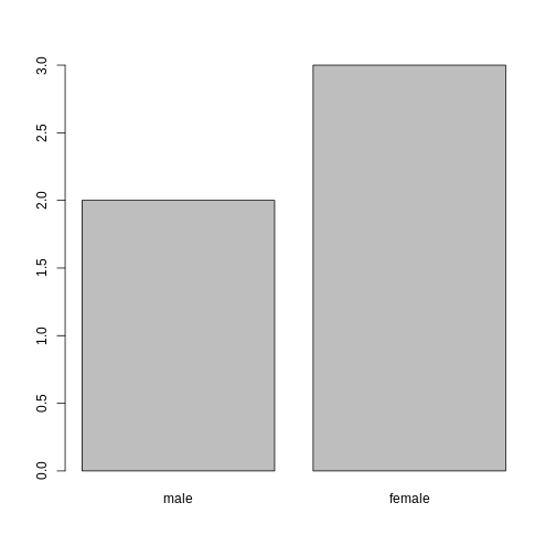
Converting to character
If you need to convert a factor to a character vector, you use
as.character(x).
R
as.character(sex)
OUTPUT
[1] "male" "female" "female" "male" "female"Renaming factors
If we want to rename these factor, it is sufficient to change its levels:
R
levels(sex)
OUTPUT
[1] "male" "female"R
levels(sex) <- c("M", "F")
sex
OUTPUT
[1] M F F M F
Levels: M F
R
plot(sex)

Challenge:
- Rename “F” and “M” to “Female” and “Male” respectively.
R
levels(sex)
OUTPUT
[1] "M" "F"R
levels(sex) <- c("Male", "Female")
Challenge:
We have seen how data frames are created when using
read.csv(), but they can also be created by hand with the
data.frame() function. There are a few mistakes in this
hand-crafted data.frame. Can you spot and fix them? Don’t
hesitate to experiment!
- missing quotations around the names of the animals
- missing one entry in the “feel” column (probably for one of the furry animals)
- missing one comma in the weight column
Challenge:
Can you predict the class for each of the columns in the following example?
Check your guesses using str(country_climate):
Are they what you expected? Why? Why not?
Try again by adding
stringsAsFactors = TRUEafter the last variable when creating the data frame. What is happening now?stringsAsFactorscan also be set when reading text-based spreadsheets into R usingread.csv().
R
country_climate <- data.frame(
       country = c("Canada", "Panama", "South Africa", "Australia"),
       climate = c("cold", "hot", "temperate", "hot/temperate"),
       temperature = c(10, 30, 18, "15"),
       northern_hemisphere = c(TRUE, TRUE, FALSE, "FALSE"),
       has_kangaroo = c(FALSE, FALSE, FALSE, 1)
       )
str(country_climate)
OUTPUT
'data.frame':	4 obs. of  5 variables:
 $ country            : chr  "Canada" "Panama" "South Africa" "Australia"
 $ climate            : chr  "cold" "hot" "temperate" "hot/temperate"
 $ temperature        : chr  "10" "30" "18" "15"
 $ northern_hemisphere: chr  "TRUE" "TRUE" "FALSE" "FALSE"
 $ has_kangaroo       : num  0 0 0 1
The automatic conversion of data type is sometimes a blessing, sometimes an annoyance. Be aware that it exists, learn the rules, and double check that data you import in R are of the correct type within your data frame. If not, use it to your advantage to detect mistakes that might have been introduced during data entry (a letter in a column that should only contain numbers for instance).
Learn more in this RStudio tutorial
Matrices
Before proceeding, now that we have learnt about data frames, let’s
recap package installation and learn about a new data type, namely the
matrix. Like a data.frame, a matrix has two
dimensions, rows and columns. But the major difference is that all cells
in a matrix must be of the same type: numeric,
character, logical, … In that respect,
matrices are closer to a vector than a
data.frame.
The default constructor for a matrix is matrix. It takes
a vector of values to populate the matrix and the number of row and/or
columns1.
The values are sorted along the columns, as illustrated below.
R
m <- matrix(1:9, ncol = 3, nrow = 3)
m
OUTPUT
     [,1] [,2] [,3]
[1,]    1    4    7
[2,]    2    5    8
[3,] 3 6 9Challenge:
Using the function installed.packages(), create a
character matrix containing the information about all
packages currently installed on your computer. Explore it.
R
## create the matrix
ip <- installed.packages()
head(ip)
## try also View(ip)
## number of package
nrow(ip)
## names of all installed packages
rownames(ip)
## type of information we have about each package
colnames(ip)
It is often useful to create large random data matrices as test data.
The exercise below asks you to create such a matrix with random data
drawn from a normal distribution of mean 0 and standard deviation 1,
which can be done with the rnorm() function.
Challenge:
Construct a matrix of dimension 1000 by 3 of normally distributed data (mean 0, standard deviation 1)
R
set.seed(123)
m <- matrix(rnorm(3000), ncol = 3)
dim(m)
OUTPUT
[1] 1000 3R
head(m)
OUTPUT
            [,1]        [,2]       [,3]
[1,] -0.56047565 -0.99579872 -0.5116037
[2,] -0.23017749 -1.03995504  0.2369379
[3,]  1.55870831 -0.01798024 -0.5415892
[4,]  0.07050839 -0.13217513  1.2192276
[5,]  0.12928774 -2.54934277  0.1741359
[6,]  1.71506499  1.04057346 -0.6152683
Formatting Dates
One of the most common issues that new (and experienced!) R users have is converting date and time information into a variable that is appropriate and usable during analyses.
Note on dates in spreadsheet programs
Dates in spreadsheets are generally stored in a single column. While this seems the most natural way to record dates, it actually is not best practice. A spreadsheet application will display the dates in a seemingly correct way (to a human observer) but how it actually handles and stores the dates may be problematic. It is often much safer to store dates with YEAR, MONTH and DAY in separate columns or as YEAR and DAY-OF-YEAR in separate columns.
Spreadsheet programs such as LibreOffice, Microsoft Excel, OpenOffice, Gnumeric, … have different (and often incompatible) ways of encoding dates (even for the same program between versions and operating systems). Additionally, Excel can turn things that aren’t dates into dates (@Zeeberg:2004), for example names or identifiers like MAR1, DEC1, OCT4. So if you’re avoiding the date format overall, it’s easier to identify these issues.
The Dates as data section of the Data Carpentry lesson provides additional insights about pitfalls of dates with spreadsheets.
We are going to use the ymd() function from the package
lubridate (which belongs to the
tidyverse; learn more on the tidyverse web site).
lubridate gets installed as part of the
tidyverse installation. When you load the
tidyverse
(library(tidyverse)), the core packages (the packages used
in most data analyses) get loaded.
lubridate however does not belong to the
core tidyverse, so you have to load it explicitly with
library(lubridate).
Start by loading the required package:
R
library("lubridate")
ymd() takes a vector representing year, month, and day,
and converts it to a Date vector. Date is a
class of data recognized by R as being a date and can be manipulated as
such. The argument that the function requires is flexible, but, as a
best practice, is a character vector formatted as “YYYY-MM-DD”.
Let’s create a date object and inspect the structure:
R
my_date <- ymd("2015-01-01")
str(my_date)
OUTPUT
Date[1:1], format: "2015-01-01"Now let’s paste the year, month, and day separately - we get the same result:
R
# sep indicates the character to use to separate each component
my_date <- ymd(paste("2015", "1", "1", sep = "-"))
str(my_date)
OUTPUT
Date[1:1], format: "2015-01-01"Let’s now familiarise ourselves with a typical date manipulation
pipeline. The small data below has stored dates in different
year, month and day columns.
R
x <- data.frame(year = c(1996, 1992, 1987, 1986, 2000, 1990, 2002, 1994, 1997, 1985),
                month = c(2,  3,  3, 10,  1,  8,  3,  4,  5,  5),
                day = c(24,  8,  1,  5,  8, 17, 13, 10, 11, 24),
                value = c(4,  5,  1,  9,  3,  8, 10,  2,  6,  7))
x
OUTPUT
   year month day value
1  1996     2  24     4
2  1992     3   8     5
3  1987     3   1     1
4  1986    10   5     9
5  2000     1   8     3
6  1990     8  17     8
7  2002     3  13    10
8  1994     4  10     2
9  1997     5  11     6
10 1985     5  24     7
Now we apply this function to the x dataset. We first
create a character vector from the year,
month, and day columns of x using
paste():
R
paste(x$year, x$month, x$day, sep = "-")
OUTPUT
 [1] "1996-2-24" "1992-3-8"  "1987-3-1"  "1986-10-5" "2000-1-8"  "1990-8-17"
 [7] "2002-3-13" "1994-4-10" "1997-5-11" "1985-5-24"
This character vector can be used as the argument for
ymd():
R
ymd(paste(x$year, x$month, x$day, sep = "-"))
OUTPUT
 [1] "1996-02-24" "1992-03-08" "1987-03-01" "1986-10-05" "2000-01-08"
 [6] "1990-08-17" "2002-03-13" "1994-04-10" "1997-05-11" "1985-05-24"
The resulting Date vector can be added to x
as a new column called date:
R
x$date <- ymd(paste(x$year, x$month, x$day, sep = "-"))
str(x) # notice the new column, with 'date' as the class
OUTPUT
'data.frame':	10 obs. of  5 variables:
 $ year : num  1996 1992 1987 1986 2000 ...
 $ month: num  2 3 3 10 1 8 3 4 5 5
 $ day  : num  24 8 1 5 8 17 13 10 11 24
 $ value: num  4 5 1 9 3 8 10 2 6 7
 $ date : Date, format: "1996-02-24" "1992-03-08" ...
Let’s make sure everything worked correctly. One way to inspect the
new column is to use summary():
R
summary(x$date)
OUTPUT
        Min.      1st Qu.       Median         Mean      3rd Qu.         Max.
"1985-05-24" "1988-01-11" "1993-03-24" "1993-03-18" "1997-01-20" "2002-03-13"
Note that ymd() expects to have the year, month and day,
in that order. If you have for instance day, month and year, you would
need dmy().
R
dmy(paste(x$day, x$month, x$year, sep = "-"))
OUTPUT
 [1] "1996-02-24" "1992-03-08" "1987-03-01" "1986-10-05" "2000-01-08"
 [6] "1990-08-17" "2002-03-13" "1994-04-10" "1997-05-11" "1985-05-24"
lubdridate has many functions to address all date
variations.
Summary of R objects
So far, we have seen several types of R object varying in the number of dimensions and whether they could store a single or multiple data types:
-
vector: one dimension (they have a length), single type of data. -
matrix: two dimensions, single type of data. -
data.frame: two dimensions, one type per column.
Lists
A data type that we haven’t seen yet, but that is useful to know, and follows from the summary that we have just seen are lists:
-
list: one dimension, every item can be of a different data type.
Below, let’s create a list containing a vector of numbers, characters, a matrix, a dataframe and another list:
R
l <- list(1:10, ## numeric
          letters, ## character
          installed.packages(), ## a matrix
          cars, ## a data.frame
          list(1, 2, 3)) ## a list
length(l)
OUTPUT
[1] 5R
str(l)
OUTPUT
List of 5
 $ : int [1:10] 1 2 3 4 5 6 7 8 9 10
 $ : chr [1:26] "a" "b" "c" "d" ...
 $ : chr [1:339, 1:17] "abind" "askpass" "backports" "base64enc" ...
  ..- attr(*, "dimnames")=List of 2
  .. ..$ : chr [1:339] "abind" "askpass" "backports" "base64enc" ...
  .. ..$ : chr [1:17] "Package" "LibPath" "Version" "Priority" ...
 $ :'data.frame':	50 obs. of  2 variables:
  ..$ speed: num [1:50] 4 4 7 7 8 9 10 10 10 11 ...
  ..$ dist : num [1:50] 2 10 4 22 16 10 18 26 34 17 ...
 $ :List of 3
  ..$ : num 1
  ..$ : num 2
  ..$ : num 3
List subsetting is done using [] to subset a new
sub-list or [[]] to extract a single element of that list
(using indices or names, if the list is named).
R
l[[1]] ## first element
OUTPUT
[1] 1 2 3 4 5 6 7 8 9 10R
l[1:2] ## a list of length 2
OUTPUT
[[1]]
 [1]  1  2  3  4  5  6  7  8  9 10

[[2]]
 [1] "a" "b" "c" "d" "e" "f" "g" "h" "i" "j" "k" "l" "m" "n" "o" "p" "q" "r" "s"
[20] "t" "u" "v" "w" "x" "y" "z"
R
l[1] ## a list of length 1
OUTPUT
[[1]]
 [1]  1  2  3  4  5  6  7  8  9 10
Exporting and saving tabular data
We have seen how to read a text-based spreadsheet into R using the
read.table family of functions. To export a
data.frame to a text-based spreadsheet, we can use the
write.table set of functions (write.csv,
write.delim, …). They all take the variable to be exported
and the file to be exported to. For example, to export the
rna data to the my_rna.csv file in the
data_output directory, we would execute:
R
write.csv(rna, file = "data_output/my_rna.csv")
This new csv file can now be shared with other collaborators who
aren’t familiar with R. Note that even though there are commas in some
of the fields in the data.frame (see for example the
“product” column), R will by default surround each field with quotes,
and thus we will be able to read it back into R correctly, despite also
using commas as column separators.
- Tabular data in R
Either the number of rows or columns are enough, as the other one can be deduced from the length of the values. Try out what happens if the values and number of rows/columns don’t add up.↩︎
Content from Manipulating and analysing data with dplyr
Last updated on 2026-07-14 | Edit this page
Overview
Questions
- Data analysis in R using the tidyverse meta-package
Objectives
- Describe the purpose of the
dplyrandtidyrpackages. - Describe several of their functions that are extremely useful to manipulate data.
- Describe the concept of a wide and a long table format, and see how to reshape a data frame from one format to the other one.
- Demonstrate how to join tables.
This episode is based on the Data Carpentries’s Data Analysis and Visualisation in R for Ecologists lesson.
Data manipulation using dplyr and
tidyr
Bracket subsetting is handy, but it can be cumbersome and difficult to read, especially for complicated operations.
Some packages can greatly facilitate our task when we manipulate
data. Packages in R are basically sets of additional functions that let
you do more stuff. The functions we’ve been using so far, like
str() or data.frame(), come built into R;
Loading packages can give you access to other specific functions. Before
you use a package for the first time you need to install it on your
machine, and then you should import it in every subsequent R session
when you need it.
The package
dplyrprovides powerful tools for data manipulation tasks. It is built to work directly with data frames, with many manipulation tasks optimised.As we will see latter on, sometimes we want a data frame to be reshaped to be able to do some specific analyses or for visualisation. The package
tidyraddresses this common problem of reshaping data and provides tools for manipulating data in a tidy way.
To learn more about dplyr and
tidyr after the workshop, you may want to
check out this handy
data transformation with dplyr
cheatsheet and this one
about tidyr.
- The
tidyversepackage is an “umbrella-package” that installs several useful packages for data analysis which work well together, such astidyr,dplyr,ggplot2,tibble, etc. These packages help us to work and interact with the data. They allow us to do many things with your data, such as subsetting, transforming, visualising, etc.
If you did the set up, you should have already installed the tidyverse package. Check to see if you have it by trying to load in from the library:
R
## load the tidyverse packages, incl. dplyr
library("tidyverse")
If you got an error message
there is no package called ‘tidyverse’ then you have not
installed the package yet for this version of R. To install the
tidyverse package type:
R
BiocManager::install("tidyverse")
If you had to install the tidyverse
package, do not forget to load it in this R session by using the
library() command above!
Loading data with tidyverse
Instead of read.csv(), we will read in our data using
the read_csv() function (notice the _ instead
of the .), from the tidyverse package
readr.
R
rna <- read_csv("data/rnaseq.csv")

## view the data
rna
OUTPUT
# A tibble: 32,428 × 19
   gene    sample  expression organism   age sex   infection strain  time tissue
   <chr>   <chr>        <dbl> <chr>    <dbl> <chr> <chr>     <chr>  <dbl> <chr>
 1 Asl     GSM254…       1170 Mus mus…     8 Fema… Influenz… C57BL…     8 Cereb…
 2 Apod    GSM254…      36194 Mus mus…     8 Fema… Influenz… C57BL…     8 Cereb…
 3 Cyp2d22 GSM254…       4060 Mus mus…     8 Fema… Influenz… C57BL…     8 Cereb…
 4 Klk6    GSM254…        287 Mus mus…     8 Fema… Influenz… C57BL…     8 Cereb…
 5 Fcrls   GSM254…         85 Mus mus…     8 Fema… Influenz… C57BL…     8 Cereb…
 6 Slc2a4  GSM254…        782 Mus mus…     8 Fema… Influenz… C57BL…     8 Cereb…
 7 Exd2    GSM254…       1619 Mus mus…     8 Fema… Influenz… C57BL…     8 Cereb…
 8 Gjc2    GSM254…        288 Mus mus…     8 Fema… Influenz… C57BL…     8 Cereb…
 9 Plp1    GSM254…      43217 Mus mus…     8 Fema… Influenz… C57BL…     8 Cereb…
10 Gnb4    GSM254…       1071 Mus mus…     8 Fema… Influenz… C57BL…     8 Cereb…
# ℹ 32,418 more rows
# ℹ 9 more variables: mouse <dbl>, ENTREZID <dbl>, product <chr>,
#   ensembl_gene_id <chr>, external_synonym <chr>, chromosome_name <chr>,
#   gene_biotype <chr>, phenotype_description <chr>,
#   hsapiens_homolog_associated_gene_name <chr>
Notice that the class of the data is now referred to as a “tibble”.
Tibbles tweak some of the behaviors of the data frame objects we introduced in the previously. The data structure is very similar to a data frame. For our purposes the only differences are that:
It displays the data type of each column under its name. Note that <
dbl> is a data type defined to hold numeric values with decimal points.It only prints the first few rows of data and only as many columns as fit on one screen.
We are now going to learn some of the most common
dplyr functions:
-
select(): subset columns -
filter(): subset rows on conditions -
mutate(): create new columns by using information from other columns -
group_by()andsummarise(): create summary statistics on grouped data -
arrange(): sort results -
count(): count discrete values
Selecting columns and filtering rows
To select columns of a data frame, use select(). The
first argument to this function is the data frame (rna),
and the subsequent arguments are the columns to keep.
R
select(rna, gene, sample, tissue, expression)
OUTPUT
# A tibble: 32,428 × 4
   gene    sample     tissue     expression
   <chr>   <chr>      <chr>           <dbl>
 1 Asl     GSM2545336 Cerebellum       1170
 2 Apod    GSM2545336 Cerebellum      36194
 3 Cyp2d22 GSM2545336 Cerebellum       4060
 4 Klk6    GSM2545336 Cerebellum        287
 5 Fcrls   GSM2545336 Cerebellum         85
 6 Slc2a4  GSM2545336 Cerebellum        782
 7 Exd2    GSM2545336 Cerebellum       1619
 8 Gjc2    GSM2545336 Cerebellum        288
 9 Plp1    GSM2545336 Cerebellum      43217
10 Gnb4    GSM2545336 Cerebellum       1071
# ℹ 32,418 more rows
To select all columns except certain ones, put a “-” in front of the variable to exclude it.
R
select(rna, -tissue, -organism)
OUTPUT
# A tibble: 32,428 × 17
   gene    sample   expression   age sex   infection strain  time mouse ENTREZID
   <chr>   <chr>         <dbl> <dbl> <chr> <chr>     <chr>  <dbl> <dbl>    <dbl>
 1 Asl     GSM2545…       1170     8 Fema… Influenz… C57BL…     8    14   109900
 2 Apod    GSM2545…      36194     8 Fema… Influenz… C57BL…     8    14    11815
 3 Cyp2d22 GSM2545…       4060     8 Fema… Influenz… C57BL…     8    14    56448
 4 Klk6    GSM2545…        287     8 Fema… Influenz… C57BL…     8    14    19144
 5 Fcrls   GSM2545…         85     8 Fema… Influenz… C57BL…     8    14    80891
 6 Slc2a4  GSM2545…        782     8 Fema… Influenz… C57BL…     8    14    20528
 7 Exd2    GSM2545…       1619     8 Fema… Influenz… C57BL…     8    14    97827
 8 Gjc2    GSM2545…        288     8 Fema… Influenz… C57BL…     8    14   118454
 9 Plp1    GSM2545…      43217     8 Fema… Influenz… C57BL…     8    14    18823
10 Gnb4    GSM2545…       1071     8 Fema… Influenz… C57BL…     8    14    14696
# ℹ 32,418 more rows
# ℹ 7 more variables: product <chr>, ensembl_gene_id <chr>,
#   external_synonym <chr>, chromosome_name <chr>, gene_biotype <chr>,
#   phenotype_description <chr>, hsapiens_homolog_associated_gene_name <chr>
This will select all the variables in rna except
tissue and organism.
To choose rows based on a specific criteria, use
filter():
R
filter(rna, sex == "Male")
OUTPUT
# A tibble: 14,740 × 19
   gene    sample  expression organism   age sex   infection strain  time tissue
   <chr>   <chr>        <dbl> <chr>    <dbl> <chr> <chr>     <chr>  <dbl> <chr>
 1 Asl     GSM254…        626 Mus mus…     8 Male  Influenz… C57BL…     4 Cereb…
 2 Apod    GSM254…      13021 Mus mus…     8 Male  Influenz… C57BL…     4 Cereb…
 3 Cyp2d22 GSM254…       2171 Mus mus…     8 Male  Influenz… C57BL…     4 Cereb…
 4 Klk6    GSM254…        448 Mus mus…     8 Male  Influenz… C57BL…     4 Cereb…
 5 Fcrls   GSM254…        180 Mus mus…     8 Male  Influenz… C57BL…     4 Cereb…
 6 Slc2a4  GSM254…        313 Mus mus…     8 Male  Influenz… C57BL…     4 Cereb…
 7 Exd2    GSM254…       2366 Mus mus…     8 Male  Influenz… C57BL…     4 Cereb…
 8 Gjc2    GSM254…        310 Mus mus…     8 Male  Influenz… C57BL…     4 Cereb…
 9 Plp1    GSM254…      53126 Mus mus…     8 Male  Influenz… C57BL…     4 Cereb…
10 Gnb4    GSM254…       1355 Mus mus…     8 Male  Influenz… C57BL…     4 Cereb…
# ℹ 14,730 more rows
# ℹ 9 more variables: mouse <dbl>, ENTREZID <dbl>, product <chr>,
#   ensembl_gene_id <chr>, external_synonym <chr>, chromosome_name <chr>,
#   gene_biotype <chr>, phenotype_description <chr>,
#   hsapiens_homolog_associated_gene_name <chr>
R
filter(rna, sex == "Male" & infection == "NonInfected")
OUTPUT
# A tibble: 4,422 × 19
   gene    sample  expression organism   age sex   infection strain  time tissue
   <chr>   <chr>        <dbl> <chr>    <dbl> <chr> <chr>     <chr>  <dbl> <chr>
 1 Asl     GSM254…        535 Mus mus…     8 Male  NonInfec… C57BL…     0 Cereb…
 2 Apod    GSM254…      13668 Mus mus…     8 Male  NonInfec… C57BL…     0 Cereb…
 3 Cyp2d22 GSM254…       2008 Mus mus…     8 Male  NonInfec… C57BL…     0 Cereb…
 4 Klk6    GSM254…       1101 Mus mus…     8 Male  NonInfec… C57BL…     0 Cereb…
 5 Fcrls   GSM254…        375 Mus mus…     8 Male  NonInfec… C57BL…     0 Cereb…
 6 Slc2a4  GSM254…        249 Mus mus…     8 Male  NonInfec… C57BL…     0 Cereb…
 7 Exd2    GSM254…       3126 Mus mus…     8 Male  NonInfec… C57BL…     0 Cereb…
 8 Gjc2    GSM254…        791 Mus mus…     8 Male  NonInfec… C57BL…     0 Cereb…
 9 Plp1    GSM254…      98658 Mus mus…     8 Male  NonInfec… C57BL…     0 Cereb…
10 Gnb4    GSM254…       2437 Mus mus…     8 Male  NonInfec… C57BL…     0 Cereb…
# ℹ 4,412 more rows
# ℹ 9 more variables: mouse <dbl>, ENTREZID <dbl>, product <chr>,
#   ensembl_gene_id <chr>, external_synonym <chr>, chromosome_name <chr>,
#   gene_biotype <chr>, phenotype_description <chr>,
#   hsapiens_homolog_associated_gene_name <chr>
Now let’s imagine we are interested in the human homologs of the
mouse genes analysed in this dataset. This information can be found in
the last column of the rna tibble, named
hsapiens_homolog_associated_gene_name. To visualise it
easily, we will create a new table containing just the 2 columns
gene and
hsapiens_homolog_associated_gene_name.
R
genes <- select(rna, gene, hsapiens_homolog_associated_gene_name)
genes
OUTPUT
# A tibble: 32,428 × 2
   gene    hsapiens_homolog_associated_gene_name
   <chr>   <chr>
 1 Asl     ASL
 2 Apod    APOD
 3 Cyp2d22 CYP2D6
 4 Klk6    KLK6
 5 Fcrls   FCRL2
 6 Slc2a4  SLC2A4
 7 Exd2    EXD2
 8 Gjc2    GJC2
 9 Plp1    PLP1
10 Gnb4    GNB4
# ℹ 32,418 more rows
Some mouse genes have no human homologs. These can be retrieved using
filter() and the is.na() function, that
determines whether something is an NA.
R
filter(genes, is.na(hsapiens_homolog_associated_gene_name))
OUTPUT
# A tibble: 4,290 × 2
   gene     hsapiens_homolog_associated_gene_name
   <chr>    <chr>
 1 Prodh    <NA>
 2 Tssk5    <NA>
 3 Vmn2r1   <NA>
 4 Gm10654  <NA>
 5 Hexa     <NA>
 6 Sult1a1  <NA>
 7 Gm6277   <NA>
 8 Tmem198b <NA>
 9 Adam1a   <NA>
10 Ebp      <NA>
# ℹ 4,280 more rows
If we want to keep only mouse genes that have a human homolog, we can
insert a “!” symbol that negates the result, so we’re asking for every
row where hsapiens_homolog_associated_gene_name is not an
NA.
R
filter(genes, !is.na(hsapiens_homolog_associated_gene_name))
OUTPUT
# A tibble: 28,138 × 2
   gene    hsapiens_homolog_associated_gene_name
   <chr>   <chr>
 1 Asl     ASL
 2 Apod    APOD
 3 Cyp2d22 CYP2D6
 4 Klk6    KLK6
 5 Fcrls   FCRL2
 6 Slc2a4  SLC2A4
 7 Exd2    EXD2
 8 Gjc2    GJC2
 9 Plp1    PLP1
10 Gnb4    GNB4
# ℹ 28,128 more rows
Pipes
What if you want to select and filter at the same time? There are three ways to do this: use intermediate steps, nested functions, or pipes.
With intermediate steps, you create a temporary data frame and use that as input to the next function, like this:
R
rna2 <- filter(rna, sex == "Male")
rna3 <- select(rna2, gene, sample, tissue, expression)
rna3
OUTPUT
# A tibble: 14,740 × 4
   gene    sample     tissue     expression
   <chr>   <chr>      <chr>           <dbl>
 1 Asl     GSM2545340 Cerebellum        626
 2 Apod    GSM2545340 Cerebellum      13021
 3 Cyp2d22 GSM2545340 Cerebellum       2171
 4 Klk6    GSM2545340 Cerebellum        448
 5 Fcrls   GSM2545340 Cerebellum        180
 6 Slc2a4  GSM2545340 Cerebellum        313
 7 Exd2    GSM2545340 Cerebellum       2366
 8 Gjc2    GSM2545340 Cerebellum        310
 9 Plp1    GSM2545340 Cerebellum      53126
10 Gnb4    GSM2545340 Cerebellum       1355
# ℹ 14,730 more rows
This is readable, but can clutter up your workspace with lots of intermediate objects that you have to name individually. With multiple steps, that can be hard to keep track of.
You can also nest functions (i.e. one function inside of another), like this:
R
rna3 <- select(filter(rna, sex == "Male"), gene, sample, tissue, expression)
rna3
OUTPUT
# A tibble: 14,740 × 4
   gene    sample     tissue     expression
   <chr>   <chr>      <chr>           <dbl>
 1 Asl     GSM2545340 Cerebellum        626
 2 Apod    GSM2545340 Cerebellum      13021
 3 Cyp2d22 GSM2545340 Cerebellum       2171
 4 Klk6    GSM2545340 Cerebellum        448
 5 Fcrls   GSM2545340 Cerebellum        180
 6 Slc2a4  GSM2545340 Cerebellum        313
 7 Exd2    GSM2545340 Cerebellum       2366
 8 Gjc2    GSM2545340 Cerebellum        310
 9 Plp1    GSM2545340 Cerebellum      53126
10 Gnb4    GSM2545340 Cerebellum       1355
# ℹ 14,730 more rows
This is handy, but can be difficult to read if too many functions are nested, as R evaluates the expression from the inside out (in this case, filtering, then selecting).
The last option, pipes, are a recent addition to R. Pipes let you take the output of one function and send it directly to the next, which is useful when you need to do many things to the same dataset.
Pipes in R look like %>% (made available via the
magrittr package) or |>
(through base R). If you use RStudio, you can type the pipe with
Ctrl + Shift + M if you have a PC or
Cmd + Shift + M if you have a Mac.
In the above code, we use the pipe to send the rna
dataset first through filter() to keep rows where
sex is Male, then through select() to keep
only the gene, sample, tissue,
and expressioncolumns.
The pipe |> takes the object on its left and passes
it directly as the first argument to the function on its right, we don’t
need to explicitly include the data frame as an argument to the
filter() and select() functions any more.
R
rna |>
  filter(sex == "Male") |>
  select(gene, sample, tissue, expression)
OUTPUT
# A tibble: 14,740 × 4
   gene    sample     tissue     expression
   <chr>   <chr>      <chr>           <dbl>
 1 Asl     GSM2545340 Cerebellum        626
 2 Apod    GSM2545340 Cerebellum      13021
 3 Cyp2d22 GSM2545340 Cerebellum       2171
 4 Klk6    GSM2545340 Cerebellum        448
 5 Fcrls   GSM2545340 Cerebellum        180
 6 Slc2a4  GSM2545340 Cerebellum        313
 7 Exd2    GSM2545340 Cerebellum       2366
 8 Gjc2    GSM2545340 Cerebellum        310
 9 Plp1    GSM2545340 Cerebellum      53126
10 Gnb4    GSM2545340 Cerebellum       1355
# ℹ 14,730 more rows
Some may find it helpful to read the pipe like the word “then”. For
instance, in the above example, we took the data frame rna,
then we filtered for rows with
sex == "Male", then we selected
columns gene, sample, tissue, and
expression.
The dplyr functions by themselves are
somewhat simple, but by combining them into linear workflows with the
pipe, we can accomplish more complex manipulations of data frames.
If we want to create a new object with this smaller version of the data, we can assign it a new name:
R
rna3 <- rna |>
  filter(sex == "Male") |>
  select(gene, sample, tissue, expression)

rna3
OUTPUT
# A tibble: 14,740 × 4
   gene    sample     tissue     expression
   <chr>   <chr>      <chr>           <dbl>
 1 Asl     GSM2545340 Cerebellum        626
 2 Apod    GSM2545340 Cerebellum      13021
 3 Cyp2d22 GSM2545340 Cerebellum       2171
 4 Klk6    GSM2545340 Cerebellum        448
 5 Fcrls   GSM2545340 Cerebellum        180
 6 Slc2a4  GSM2545340 Cerebellum        313
 7 Exd2    GSM2545340 Cerebellum       2366
 8 Gjc2    GSM2545340 Cerebellum        310
 9 Plp1    GSM2545340 Cerebellum      53126
10 Gnb4    GSM2545340 Cerebellum       1355
# ℹ 14,730 more rowsChallenge:
Using pipes, subset the rna data to keep observations in
female mice at time 0, where the gene has an expression higher than
50000, and retain only the columns gene,
sample, time, expression and
age.
R
rna |>
  filter(expression > 50000,
         sex == "Female",
         time == 0 ) |>
  select(gene, sample, time, expression, age)
OUTPUT
# A tibble: 9 × 5
  gene   sample      time expression   age
  <chr>  <chr>      <dbl>      <dbl> <dbl>
1 Plp1   GSM2545337     0     101241     8
2 Atp1b1 GSM2545337     0      53260     8
3 Plp1   GSM2545338     0      96534     8
4 Atp1b1 GSM2545338     0      50614     8
5 Plp1   GSM2545348     0     102790     8
6 Atp1b1 GSM2545348     0      59544     8
7 Plp1   GSM2545353     0      71237     8
8 Glul   GSM2545353     0      52451     8
9 Atp1b1 GSM2545353     0      61451     8
Mutate
Frequently you’ll want to create new columns based on the values of
existing columns, for example to do unit conversions, or to find the
ratio of values in two columns. For this we’ll use
mutate().
To create a new column of time in hours:
R
rna |>
  mutate(time_hours = time * 24) |>
  select(time, time_hours)
OUTPUT
# A tibble: 32,428 × 2
    time time_hours
   <dbl>      <dbl>
 1     8        192
 2     8        192
 3     8        192
 4     8        192
 5     8        192
 6     8        192
 7     8        192
 8     8        192
 9     8        192
10     8        192
# ℹ 32,418 more rows
You can also create a second new column based on the first new column
within the same call of mutate():
R
rna |>
  mutate(time_hours = time * 24,
         time_mn = time_hours * 60) |>
  select(time, time_hours, time_mn)
OUTPUT
# A tibble: 32,428 × 3
    time time_hours time_mn
   <dbl>      <dbl>   <dbl>
 1     8        192   11520
 2     8        192   11520
 3     8        192   11520
 4     8        192   11520
 5     8        192   11520
 6     8        192   11520
 7     8        192   11520
 8     8        192   11520
 9     8        192   11520
10     8        192   11520
# ℹ 32,418 more rows
Challenge
Create a new data frame from the rna data that meets the
following criteria: contains only the gene,
chromosome_name, phenotype_description,
sample, and expression columns. The expression
values should be log-transformed. This data frame must only contain
genes located on sex chromosomes, associated with a
phenotype_description, and with a log expression higher than 5.
Hint: think about how the commands should be ordered to produce this data frame!
R
rna |>
  mutate(expression = log(expression)) |>
  select(gene, chromosome_name, phenotype_description, sample, expression) |>
  filter(chromosome_name == "X" | chromosome_name == "Y") |>
  filter(!is.na(phenotype_description)) |>
  filter(expression > 5)
OUTPUT
# A tibble: 649 × 5
   gene   chromosome_name phenotype_description                sample expression
   <chr>  <chr>           <chr>                                <chr>       <dbl>
 1 Plp1   X               abnormal CNS glial cell morphology   GSM25…      10.7
 2 Slc7a3 X               decreased body length                GSM25…       5.46
 3 Plxnb3 X               abnormal coat appearance             GSM25…       6.58
 4 Rbm3   X               abnormal liver morphology            GSM25…       9.32
 5 Cfp    X               abnormal cardiovascular system phys… GSM25…       6.18
 6 Ebp    X               abnormal embryonic erythrocyte morp… GSM25…       6.68
 7 Cd99l2 X               abnormal cellular extravasation      GSM25…       8.04
 8 Piga   X               abnormal brain development           GSM25…       6.06
 9 Pim2   X               decreased T cell proliferation       GSM25…       7.11
10 Itm2a  X               no abnormal phenotype detected       GSM25…       7.48
# ℹ 639 more rows
Split-apply-combine data analysis
Many data analysis tasks can be approached using the
split-apply-combine paradigm: split the data into groups, apply
some analysis to each group, and then combine the results.
dplyr makes this very easy through the use
of the group_by() function.
R
rna |>
  group_by(gene)
OUTPUT
# A tibble: 32,428 × 19
# Groups:   gene [1,474]
   gene    sample  expression organism   age sex   infection strain  time tissue
   <chr>   <chr>        <dbl> <chr>    <dbl> <chr> <chr>     <chr>  <dbl> <chr>
 1 Asl     GSM254…       1170 Mus mus…     8 Fema… Influenz… C57BL…     8 Cereb…
 2 Apod    GSM254…      36194 Mus mus…     8 Fema… Influenz… C57BL…     8 Cereb…
 3 Cyp2d22 GSM254…       4060 Mus mus…     8 Fema… Influenz… C57BL…     8 Cereb…
 4 Klk6    GSM254…        287 Mus mus…     8 Fema… Influenz… C57BL…     8 Cereb…
 5 Fcrls   GSM254…         85 Mus mus…     8 Fema… Influenz… C57BL…     8 Cereb…
 6 Slc2a4  GSM254…        782 Mus mus…     8 Fema… Influenz… C57BL…     8 Cereb…
 7 Exd2    GSM254…       1619 Mus mus…     8 Fema… Influenz… C57BL…     8 Cereb…
 8 Gjc2    GSM254…        288 Mus mus…     8 Fema… Influenz… C57BL…     8 Cereb…
 9 Plp1    GSM254…      43217 Mus mus…     8 Fema… Influenz… C57BL…     8 Cereb…
10 Gnb4    GSM254…       1071 Mus mus…     8 Fema… Influenz… C57BL…     8 Cereb…
# ℹ 32,418 more rows
# ℹ 9 more variables: mouse <dbl>, ENTREZID <dbl>, product <chr>,
#   ensembl_gene_id <chr>, external_synonym <chr>, chromosome_name <chr>,
#   gene_biotype <chr>, phenotype_description <chr>,
#   hsapiens_homolog_associated_gene_name <chr>
The group_by() function doesn’t perform any data
processing, it groups the data into subsets: in the example above, our
initial tibble of 32428 observations is split into 1474
groups based on the gene variable.
We could similarly decide to group the tibble by the samples:
R
rna |>
  group_by(sample)
OUTPUT
# A tibble: 32,428 × 19
# Groups:   sample [22]
   gene    sample  expression organism   age sex   infection strain  time tissue
   <chr>   <chr>        <dbl> <chr>    <dbl> <chr> <chr>     <chr>  <dbl> <chr>
 1 Asl     GSM254…       1170 Mus mus…     8 Fema… Influenz… C57BL…     8 Cereb…
 2 Apod    GSM254…      36194 Mus mus…     8 Fema… Influenz… C57BL…     8 Cereb…
 3 Cyp2d22 GSM254…       4060 Mus mus…     8 Fema… Influenz… C57BL…     8 Cereb…
 4 Klk6    GSM254…        287 Mus mus…     8 Fema… Influenz… C57BL…     8 Cereb…
 5 Fcrls   GSM254…         85 Mus mus…     8 Fema… Influenz… C57BL…     8 Cereb…
 6 Slc2a4  GSM254…        782 Mus mus…     8 Fema… Influenz… C57BL…     8 Cereb…
 7 Exd2    GSM254…       1619 Mus mus…     8 Fema… Influenz… C57BL…     8 Cereb…
 8 Gjc2    GSM254…        288 Mus mus…     8 Fema… Influenz… C57BL…     8 Cereb…
 9 Plp1    GSM254…      43217 Mus mus…     8 Fema… Influenz… C57BL…     8 Cereb…
10 Gnb4    GSM254…       1071 Mus mus…     8 Fema… Influenz… C57BL…     8 Cereb…
# ℹ 32,418 more rows
# ℹ 9 more variables: mouse <dbl>, ENTREZID <dbl>, product <chr>,
#   ensembl_gene_id <chr>, external_synonym <chr>, chromosome_name <chr>,
#   gene_biotype <chr>, phenotype_description <chr>,
#   hsapiens_homolog_associated_gene_name <chr>
Here our initial tibble of 32428 observations is split
into 22 groups based on the sample variable.
Once the data has been grouped, subsequent operations will be applied on each group independently.
The summarise() function
group_by() is often used together with
summarise(), which collapses each group into a single-row
summary of that group.
group_by() takes as arguments the column names that
contain the categorical variables for which you want to
calculate the summary statistics. So to compute the mean
expression by gene:
R
rna |>
  group_by(gene) |>
  summarise(mean_expression = mean(expression))
OUTPUT
# A tibble: 1,474 × 2
   gene     mean_expression
   <chr>              <dbl>
 1 AI504432         1053.
 2 AW046200          131.
 3 AW551984          295.
 4 Aamp             4751.
 5 Abca12              4.55
 6 Abcc8            2498.
 7 Abhd14a           525.
 8 Abi2             4909.
 9 Abi3bp           1002.
10 Abl2             2124.
# ℹ 1,464 more rows
We could also want to calculate the mean expression levels of all genes in each sample:
R
rna |>
  group_by(sample) |>
  summarise(mean_expression = mean(expression))
OUTPUT
# A tibble: 22 × 2
   sample     mean_expression
   <chr>                <dbl>
 1 GSM2545336           2062.
 2 GSM2545337           1766.
 3 GSM2545338           1668.
 4 GSM2545339           1696.
 5 GSM2545340           1682.
 6 GSM2545341           1638.
 7 GSM2545342           1594.
 8 GSM2545343           2107.
 9 GSM2545344           1712.
10 GSM2545345           1700.
# ℹ 12 more rows
But we can can also group by multiple columns:
R
rna |>
  group_by(gene, infection, time) |>
  summarise(mean_expression = mean(expression))
OUTPUT
`summarise()` has regrouped the output.
ℹ Summaries were computed grouped by gene, infection, and time.
ℹ Output is grouped by gene and infection.
ℹ Use `summarise(.groups = "drop_last")` to silence this message.
ℹ Use `summarise(.by = c(gene, infection, time))` for per-operation grouping
  (`?dplyr::dplyr_by`) instead.
OUTPUT
# A tibble: 4,422 × 4
# Groups:   gene, infection [2,948]
   gene     infection    time mean_expression
   <chr>    <chr>       <dbl>           <dbl>
 1 AI504432 InfluenzaA      4           1104.
 2 AI504432 InfluenzaA      8           1014
 3 AI504432 NonInfected     0           1034.
 4 AW046200 InfluenzaA      4            152.
 5 AW046200 InfluenzaA      8             81
 6 AW046200 NonInfected     0            155.
 7 AW551984 InfluenzaA      4            302.
 8 AW551984 InfluenzaA      8            342.
 9 AW551984 NonInfected     0            238
10 Aamp     InfluenzaA      4           4870
# ℹ 4,412 more rows
Once the data is grouped, you can also summarise multiple variables
at the same time (and not necessarily on the same variable). For
instance, we could add a column indicating the median
expression by gene and by condition:
R
rna |>
  group_by(gene, infection, time) |>
  summarise(mean_expression = mean(expression),
            median_expression = median(expression))
OUTPUT
`summarise()` has regrouped the output.
ℹ Summaries were computed grouped by gene, infection, and time.
ℹ Output is grouped by gene and infection.
ℹ Use `summarise(.groups = "drop_last")` to silence this message.
ℹ Use `summarise(.by = c(gene, infection, time))` for per-operation grouping
  (`?dplyr::dplyr_by`) instead.
OUTPUT
# A tibble: 4,422 × 5
# Groups:   gene, infection [2,948]
   gene     infection    time mean_expression median_expression
   <chr>    <chr>       <dbl>           <dbl>             <dbl>
 1 AI504432 InfluenzaA      4           1104.             1094.
 2 AI504432 InfluenzaA      8           1014               985
 3 AI504432 NonInfected     0           1034.             1016
 4 AW046200 InfluenzaA      4            152.              144.
 5 AW046200 InfluenzaA      8             81                82
 6 AW046200 NonInfected     0            155.              163
 7 AW551984 InfluenzaA      4            302.              245
 8 AW551984 InfluenzaA      8            342.              287
 9 AW551984 NonInfected     0            238               265
10 Aamp     InfluenzaA      4           4870              4708
# ℹ 4,412 more rows
Challenge
Calculate the mean expression level of gene “Dok3” by timepoints.
R
rna |>
  filter(gene == "Dok3") |>
  group_by(time) |>
  summarise(mean = mean(expression))
OUTPUT
# A tibble: 3 × 2
   time  mean
  <dbl> <dbl>
1     0  169
2     4  156.
3     8   61
Counting
When working with data, we often want to know the number of
observations found for each factor or combination of factors. For this
task, dplyr provides count().
For example, if we wanted to count the number of rows of data for each
infected and non-infected samples, we would do:
R
rna |>
    count(infection)
OUTPUT
# A tibble: 2 × 2
  infection       n
  <chr>       <int>
1 InfluenzaA  22110
2 NonInfected 10318
The count() function is shorthand for something we’ve
already seen: grouping by a variable, and summarising it by counting the
number of observations in that group. In other words,
rna |> count(infection) is equivalent to:
R
rna |>
    group_by(infection) |>
    summarise(n = n())
OUTPUT
# A tibble: 2 × 2
  infection       n
  <chr>       <int>
1 InfluenzaA  22110
2 NonInfected 10318
The previous example shows the use of count() to count
the number of rows/observations for one factor (i.e.,
infection). If we wanted to count a combination of
factors, such as infection and time, we
would specify the first and the second factor as the arguments of
count():
R
rna |>
    count(infection, time)
OUTPUT
# A tibble: 3 × 3
  infection    time     n
  <chr>       <dbl> <int>
1 InfluenzaA      4 11792
2 InfluenzaA      8 10318
3 NonInfected     0 10318
which is equivalent to this:
R
rna |>
  group_by(infection, time) |>
  summarise(n = n())
OUTPUT
`summarise()` has regrouped the output.
ℹ Summaries were computed grouped by infection and time.
ℹ Output is grouped by infection.
ℹ Use `summarise(.groups = "drop_last")` to silence this message.
ℹ Use `summarise(.by = c(infection, time))` for per-operation grouping
  (`?dplyr::dplyr_by`) instead.
OUTPUT
# A tibble: 3 × 3
# Groups:   infection [2]
  infection    time     n
  <chr>       <dbl> <int>
1 InfluenzaA      4 11792
2 InfluenzaA      8 10318
3 NonInfected     0 10318
It is sometimes useful to sort the result to facilitate the
comparisons. We can use arrange() to sort the table. For
instance, we might want to arrange the table above by time:
R
rna |>
  count(infection, time) |>
  arrange(time)
OUTPUT
# A tibble: 3 × 3
  infection    time     n
  <chr>       <dbl> <int>
1 NonInfected     0 10318
2 InfluenzaA      4 11792
3 InfluenzaA      8 10318
or by counts:
R
rna |>
  count(infection, time) |>
  arrange(n)
OUTPUT
# A tibble: 3 × 3
  infection    time     n
  <chr>       <dbl> <int>
1 InfluenzaA      8 10318
2 NonInfected     0 10318
3 InfluenzaA      4 11792
To sort in descending order, we need to add the desc()
function:
R
rna |>
  count(infection, time) |>
  arrange(desc(n))
OUTPUT
# A tibble: 3 × 3
  infection    time     n
  <chr>       <dbl> <int>
1 InfluenzaA      4 11792
2 InfluenzaA      8 10318
3 NonInfected     0 10318
Challenge
- How many genes were analysed in each sample?
- Use
group_by()andsummarise()to evaluate the sequencing depth (the sum of all counts) in each sample. Which sample has the highest sequencing depth? - Pick one sample and evaluate the number of genes by biotype.
- Identify genes associated with the “abnormal DNA methylation” phenotype description, and calculate their mean expression (in log) at time 0, time 4 and time 8.
R
## 1.
rna |>
  count(sample)
OUTPUT
# A tibble: 22 × 2
   sample         n
   <chr>      <int>
 1 GSM2545336  1474
 2 GSM2545337  1474
 3 GSM2545338  1474
 4 GSM2545339  1474
 5 GSM2545340  1474
 6 GSM2545341  1474
 7 GSM2545342  1474
 8 GSM2545343  1474
 9 GSM2545344  1474
10 GSM2545345  1474
# ℹ 12 more rows
R
## 2.
rna |>
  group_by(sample) |>
  summarise(seq_depth = sum(expression)) |>
  arrange(desc(seq_depth))
OUTPUT
# A tibble: 22 × 2
   sample     seq_depth
   <chr>          <dbl>
 1 GSM2545350   3255566
 2 GSM2545352   3216163
 3 GSM2545343   3105652
 4 GSM2545336   3039671
 5 GSM2545380   3036098
 6 GSM2545353   2953249
 7 GSM2545348   2913678
 8 GSM2545362   2913517
 9 GSM2545351   2782464
10 GSM2545349   2758006
# ℹ 12 more rows
R
## 3.
rna |>
  filter(sample == "GSM2545336") |>
  count(gene_biotype) |>
  arrange(desc(n))
OUTPUT
# A tibble: 13 × 2
   gene_biotype                           n
   <chr>                              <int>
 1 protein_coding                      1321
 2 lncRNA                                69
 3 processed_pseudogene                  59
 4 miRNA                                  7
 5 snoRNA                                 5
 6 TEC                                    4
 7 polymorphic_pseudogene                 2
 8 unprocessed_pseudogene                 2
 9 IG_C_gene                              1
10 scaRNA                                 1
11 transcribed_processed_pseudogene       1
12 transcribed_unitary_pseudogene         1
13 transcribed_unprocessed_pseudogene     1
R
## 4.
rna |>
  filter(phenotype_description == "abnormal DNA methylation") |>
  group_by(gene, time) |>
  summarise(mean_expression = mean(log(expression))) |>
  arrange()
OUTPUT
`summarise()` has regrouped the output.
ℹ Summaries were computed grouped by gene and time.
ℹ Output is grouped by gene.
ℹ Use `summarise(.groups = "drop_last")` to silence this message.
ℹ Use `summarise(.by = c(gene, time))` for per-operation grouping
  (`?dplyr::dplyr_by`) instead.
OUTPUT
# A tibble: 6 × 3
# Groups:   gene [2]
  gene   time mean_expression
  <chr> <dbl>           <dbl>
1 Xist      0            6.95
2 Xist      4            6.34
3 Xist      8            7.13
4 Zdbf2     0            6.27
5 Zdbf2     4            6.27
6 Zdbf2     8            6.19
Reshaping data
In the rna tibble, the rows contain expression values
(the unit) that are associated with a combination of 2 other variables:
gene and sample.
All the other columns correspond to variables describing either the sample (organism, age, sex, …) or the gene (gene_biotype, ENTREZ_ID, product, …). The variables that don’t change with genes or with samples will have the same value in all the rows.
R
rna |>
  arrange(gene)
OUTPUT
# A tibble: 32,428 × 19
   gene     sample expression organism   age sex   infection strain  time tissue
   <chr>    <chr>       <dbl> <chr>    <dbl> <chr> <chr>     <chr>  <dbl> <chr>
 1 AI504432 GSM25…       1230 Mus mus…     8 Fema… Influenz… C57BL…     8 Cereb…
 2 AI504432 GSM25…       1085 Mus mus…     8 Fema… NonInfec… C57BL…     0 Cereb…
 3 AI504432 GSM25…        969 Mus mus…     8 Fema… NonInfec… C57BL…     0 Cereb…
 4 AI504432 GSM25…       1284 Mus mus…     8 Fema… Influenz… C57BL…     4 Cereb…
 5 AI504432 GSM25…        966 Mus mus…     8 Male  Influenz… C57BL…     4 Cereb…
 6 AI504432 GSM25…        918 Mus mus…     8 Male  Influenz… C57BL…     8 Cereb…
 7 AI504432 GSM25…        985 Mus mus…     8 Fema… Influenz… C57BL…     8 Cereb…
 8 AI504432 GSM25…        972 Mus mus…     8 Male  NonInfec… C57BL…     0 Cereb…
 9 AI504432 GSM25…       1000 Mus mus…     8 Fema… Influenz… C57BL…     4 Cereb…
10 AI504432 GSM25…        816 Mus mus…     8 Male  Influenz… C57BL…     4 Cereb…
# ℹ 32,418 more rows
# ℹ 9 more variables: mouse <dbl>, ENTREZID <dbl>, product <chr>,
#   ensembl_gene_id <chr>, external_synonym <chr>, chromosome_name <chr>,
#   gene_biotype <chr>, phenotype_description <chr>,
#   hsapiens_homolog_associated_gene_name <chr>
This structure is called a long-format, as one column
contains all the values, and other column(s) list(s) the context of the
value.
In certain cases, the long-format is not really
“human-readable”, and another format, a wide-format is
preferred, as a more compact way of representing the data. This is
typically the case with gene expression values that scientists are used
to look as matrices, were rows represent genes and columns represent
samples.
In this format, it would therefore become straightforward to explore the relationship between the gene expression levels within, and between, the samples.
OUTPUT
# A tibble: 1,474 × 23
   gene    GSM2545336 GSM2545337 GSM2545338 GSM2545339 GSM2545340 GSM2545341
   <chr>        <dbl>      <dbl>      <dbl>      <dbl>      <dbl>      <dbl>
 1 Asl           1170        361        400        586        626        988
 2 Apod         36194      10347       9173      10620      13021      29594
 3 Cyp2d22       4060       1616       1603       1901       2171       3349
 4 Klk6           287        629        641        578        448        195
 5 Fcrls           85        233        244        237        180         38
 6 Slc2a4         782        231        248        265        313        786
 7 Exd2          1619       2288       2235       2513       2366       1359
 8 Gjc2           288        595        568        551        310        146
 9 Plp1         43217     101241      96534      58354      53126      27173
10 Gnb4          1071       1791       1867       1430       1355        798
# ℹ 1,464 more rows
# ℹ 16 more variables: GSM2545342 <dbl>, GSM2545343 <dbl>, GSM2545344 <dbl>,
#   GSM2545345 <dbl>, GSM2545346 <dbl>, GSM2545347 <dbl>, GSM2545348 <dbl>,
#   GSM2545349 <dbl>, GSM2545350 <dbl>, GSM2545351 <dbl>, GSM2545352 <dbl>,
#   GSM2545353 <dbl>, GSM2545354 <dbl>, GSM2545362 <dbl>, GSM2545363 <dbl>,
#   GSM2545380 <dbl>
To convert the gene expression values from rna into a
wide-format, we need to create a new table where the values of the
sample column would become the names of column
variables.
The key point here is that we are still following a tidy data structure, but we have reshaped the data according to the observations of interest: expression levels per gene instead of recording them per gene and per sample.
The opposite transformation would be to transform column names into values of a new variable.
We can do both these of transformations with two tidyr
functions, pivot_longer() and pivot_wider()
(see the article about pivots on the
tidyr website for details).
Pivoting the data into a wider format
Let’s select the first 3 columns of rna and use
pivot_wider() to transform the data into a wide-format.
R
rna_exp <- rna |>
  select(gene, sample, expression)
rna_exp
OUTPUT
# A tibble: 32,428 × 3
   gene    sample     expression
   <chr>   <chr>           <dbl>
 1 Asl     GSM2545336       1170
 2 Apod    GSM2545336      36194
 3 Cyp2d22 GSM2545336       4060
 4 Klk6    GSM2545336        287
 5 Fcrls   GSM2545336         85
 6 Slc2a4  GSM2545336        782
 7 Exd2    GSM2545336       1619
 8 Gjc2    GSM2545336        288
 9 Plp1    GSM2545336      43217
10 Gnb4    GSM2545336       1071
# ℹ 32,418 more rows
pivot_wider takes three main arguments:
- the data to be transformed;
- the
names_from: the column whose values will become new column names; - the
values_from: the column whose values will fill the new columns.
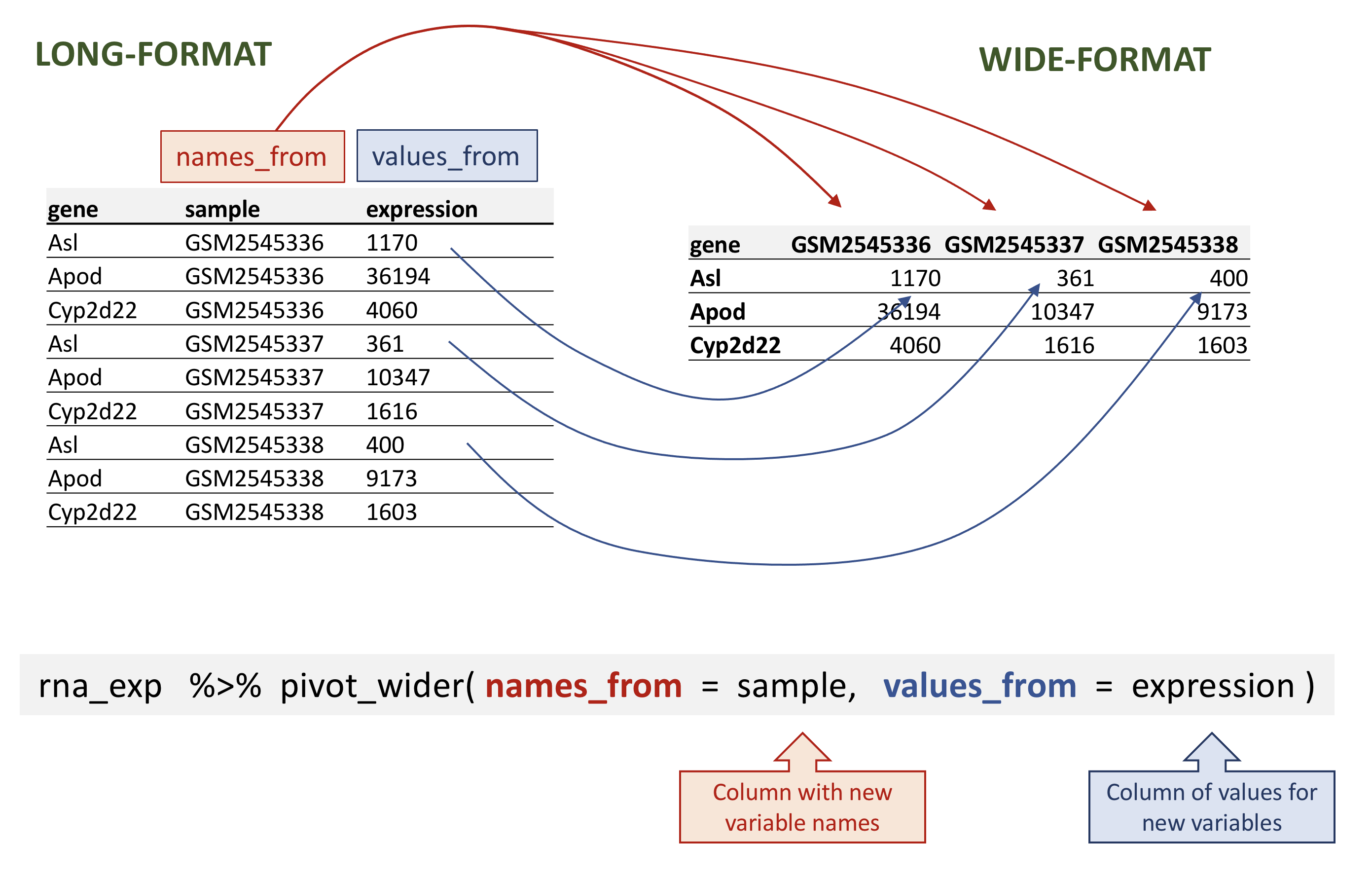
rna data.
R
rna_wide <- rna_exp |>
  pivot_wider(names_from = sample,
              values_from = expression)
rna_wide
OUTPUT
# A tibble: 1,474 × 23
   gene    GSM2545336 GSM2545337 GSM2545338 GSM2545339 GSM2545340 GSM2545341
   <chr>        <dbl>      <dbl>      <dbl>      <dbl>      <dbl>      <dbl>
 1 Asl           1170        361        400        586        626        988
 2 Apod         36194      10347       9173      10620      13021      29594
 3 Cyp2d22       4060       1616       1603       1901       2171       3349
 4 Klk6           287        629        641        578        448        195
 5 Fcrls           85        233        244        237        180         38
 6 Slc2a4         782        231        248        265        313        786
 7 Exd2          1619       2288       2235       2513       2366       1359
 8 Gjc2           288        595        568        551        310        146
 9 Plp1         43217     101241      96534      58354      53126      27173
10 Gnb4          1071       1791       1867       1430       1355        798
# ℹ 1,464 more rows
# ℹ 16 more variables: GSM2545342 <dbl>, GSM2545343 <dbl>, GSM2545344 <dbl>,
#   GSM2545345 <dbl>, GSM2545346 <dbl>, GSM2545347 <dbl>, GSM2545348 <dbl>,
#   GSM2545349 <dbl>, GSM2545350 <dbl>, GSM2545351 <dbl>, GSM2545352 <dbl>,
#   GSM2545353 <dbl>, GSM2545354 <dbl>, GSM2545362 <dbl>, GSM2545363 <dbl>,
#   GSM2545380 <dbl>
Note that by default, the pivot_wider() function will
add NA for missing values.
Let’s imagine that for some reason, we had some missing expression values for some genes in certain samples. In the following fictive example, the gene Cyp2d22 has only one expression value, in GSM2545338 sample.
R
rna_with_missing_values <- rna |>
  select(gene, sample, expression) |>
  filter(gene %in% c("Asl", "Apod", "Cyp2d22")) |>
  filter(sample %in% c("GSM2545336", "GSM2545337", "GSM2545338")) |>
  arrange(sample) |>
  filter(!(gene == "Cyp2d22" & sample != "GSM2545338"))
rna_with_missing_values
OUTPUT
# A tibble: 7 × 3
  gene    sample     expression
  <chr>   <chr>           <dbl>
1 Asl     GSM2545336       1170
2 Apod    GSM2545336      36194
3 Asl     GSM2545337        361
4 Apod    GSM2545337      10347
5 Asl     GSM2545338        400
6 Apod    GSM2545338       9173
7 Cyp2d22 GSM2545338       1603
By default, the pivot_wider() function will add
NA for missing values. This can be parameterised with the
values_fill argument of the pivot_wider()
function.
R
rna_with_missing_values |>
  pivot_wider(names_from = sample,
              values_from = expression)
OUTPUT
# A tibble: 3 × 4
  gene    GSM2545336 GSM2545337 GSM2545338
  <chr>        <dbl>      <dbl>      <dbl>
1 Asl           1170        361        400
2 Apod         36194      10347       9173
3 Cyp2d22         NA         NA       1603
R
rna_with_missing_values |>
  pivot_wider(names_from = sample,
              values_from = expression,
              values_fill = 0)
OUTPUT
# A tibble: 3 × 4
  gene    GSM2545336 GSM2545337 GSM2545338
  <chr>        <dbl>      <dbl>      <dbl>
1 Asl           1170        361        400
2 Apod         36194      10347       9173
3 Cyp2d22          0          0       1603
Pivoting data into a longer format
In the opposite situation we are using the column names and turning them into a pair of new variables. One variable represents the column names as values, and the other variable contains the values previously associated with the column names.
pivot_longer() takes four main arguments:
- the data to be transformed;
- the
names_to: the new column name we wish to create and populate with the current column names; - the
values_to: the new column name we wish to create and populate with current values; - the names of the columns to be used to populate the
names_toandvalues_tovariables (or to drop).
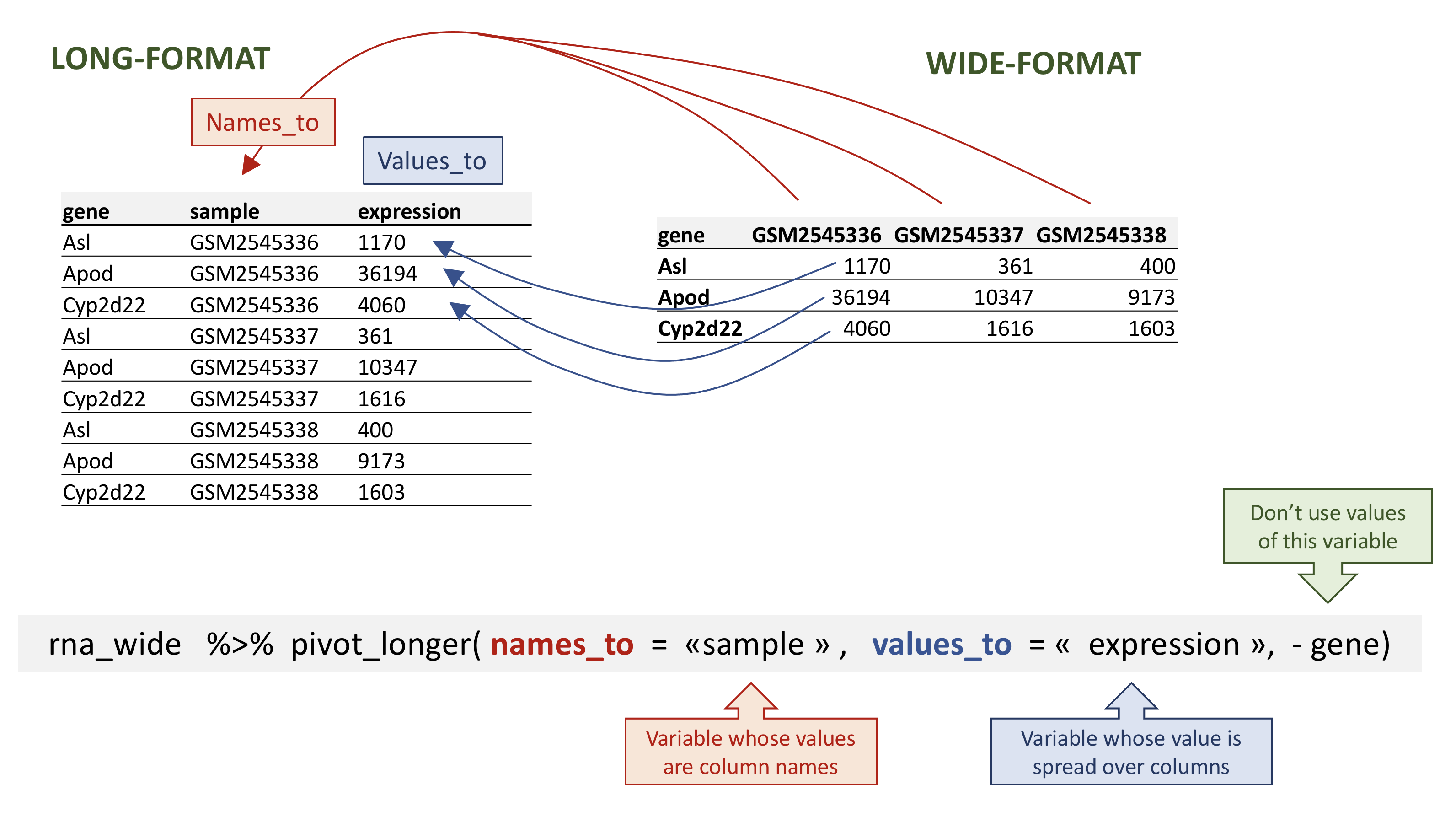
rna data.
To recreate rna_long from rna_wide we would
create a key called sample and value called
expression and use all columns except gene for
the key variable. Here we drop gene column with a minus
sign.
Notice how the new variable names are to be quoted here.
R
rna_long <- rna_wide |>
    pivot_longer(names_to = "sample",
                 values_to = "expression",
                 -gene)
rna_long
OUTPUT
# A tibble: 32,428 × 3
   gene  sample     expression
   <chr> <chr>           <dbl>
 1 Asl   GSM2545336       1170
 2 Asl   GSM2545337        361
 3 Asl   GSM2545338        400
 4 Asl   GSM2545339        586
 5 Asl   GSM2545340        626
 6 Asl   GSM2545341        988
 7 Asl   GSM2545342        836
 8 Asl   GSM2545343        535
 9 Asl   GSM2545344        586
10 Asl   GSM2545345        597
# ℹ 32,418 more rows
We could also have used a specification for what columns to include.
This can be useful if you have a large number of identifying columns,
and it’s easier to specify what to gather than what to leave alone. Here
the starts_with() function can help to retrieve sample
names without having to list them all! Another possibility would be to
use the : operator!
R
rna_wide |>
    pivot_longer(names_to = "sample",
                 values_to = "expression",
                 cols = starts_with("GSM"))
OUTPUT
# A tibble: 32,428 × 3
   gene  sample     expression
   <chr> <chr>           <dbl>
 1 Asl   GSM2545336       1170
 2 Asl   GSM2545337        361
 3 Asl   GSM2545338        400
 4 Asl   GSM2545339        586
 5 Asl   GSM2545340        626
 6 Asl   GSM2545341        988
 7 Asl   GSM2545342        836
 8 Asl   GSM2545343        535
 9 Asl   GSM2545344        586
10 Asl   GSM2545345        597
# ℹ 32,418 more rows
R
rna_wide |>
    pivot_longer(names_to = "sample",
                 values_to = "expression",
                 GSM2545336:GSM2545380)
OUTPUT
# A tibble: 32,428 × 3
   gene  sample     expression
   <chr> <chr>           <dbl>
 1 Asl   GSM2545336       1170
 2 Asl   GSM2545337        361
 3 Asl   GSM2545338        400
 4 Asl   GSM2545339        586
 5 Asl   GSM2545340        626
 6 Asl   GSM2545341        988
 7 Asl   GSM2545342        836
 8 Asl   GSM2545343        535
 9 Asl   GSM2545344        586
10 Asl   GSM2545345        597
# ℹ 32,418 more rows
Note that if we had missing values in the wide-format, the
NA would be included in the new long format.
Remember our previous fictive tibble containing missing values:
R
rna_with_missing_values
OUTPUT
# A tibble: 7 × 3
  gene    sample     expression
  <chr>   <chr>           <dbl>
1 Asl     GSM2545336       1170
2 Apod    GSM2545336      36194
3 Asl     GSM2545337        361
4 Apod    GSM2545337      10347
5 Asl     GSM2545338        400
6 Apod    GSM2545338       9173
7 Cyp2d22 GSM2545338       1603
R
wide_with_NA <- rna_with_missing_values |>
  pivot_wider(names_from = sample,
              values_from = expression)
wide_with_NA
OUTPUT
# A tibble: 3 × 4
  gene    GSM2545336 GSM2545337 GSM2545338
  <chr>        <dbl>      <dbl>      <dbl>
1 Asl           1170        361        400
2 Apod         36194      10347       9173
3 Cyp2d22         NA         NA       1603
R
wide_with_NA |>
    pivot_longer(names_to = "sample",
                 values_to = "expression",
                 -gene)
OUTPUT
# A tibble: 9 × 3
  gene    sample     expression
  <chr>   <chr>           <dbl>
1 Asl     GSM2545336       1170
2 Asl     GSM2545337        361
3 Asl     GSM2545338        400
4 Apod    GSM2545336      36194
5 Apod    GSM2545337      10347
6 Apod    GSM2545338       9173
7 Cyp2d22 GSM2545336         NA
8 Cyp2d22 GSM2545337         NA
9 Cyp2d22 GSM2545338       1603
Pivoting to wider and longer formats can be a useful way to balance out a dataset so every replicate has the same composition.
Question
Starting from the rna table, use the pivot_wider()
function to create a wide-format table giving the gene expression levels
in each mouse. Then use the pivot_longer() function to
restore a long-format table.
R
rna1 <- rna |>
select(gene, mouse, expression) |>
pivot_wider(names_from = mouse, values_from = expression)
rna1
OUTPUT
# A tibble: 1,474 × 23
   gene     `14`    `9`  `10`  `15`  `18`   `6`   `5`  `11`  `22`  `13`  `23`
   <chr>   <dbl>  <dbl> <dbl> <dbl> <dbl> <dbl> <dbl> <dbl> <dbl> <dbl> <dbl>
 1 Asl      1170    361   400   586   626   988   836   535   586   597   938
 2 Apod    36194  10347  9173 10620 13021 29594 24959 13668 13230 15868 27769
 3 Cyp2d22  4060   1616  1603  1901  2171  3349  3122  2008  2254  2277  2985
 4 Klk6      287    629   641   578   448   195   186  1101   537   567   327
 5 Fcrls      85    233   244   237   180    38    68   375   199   177    89
 6 Slc2a4    782    231   248   265   313   786   528   249   266   357   654
 7 Exd2     1619   2288  2235  2513  2366  1359  1474  3126  2379  2173  1531
 8 Gjc2      288    595   568   551   310   146   186   791   454   370   240
 9 Plp1    43217 101241 96534 58354 53126 27173 28728 98658 61356 61647 38019
10 Gnb4     1071   1791  1867  1430  1355   798   806  2437  1394  1554   960
# ℹ 1,464 more rows
# ℹ 11 more variables: `24` <dbl>, `8` <dbl>, `7` <dbl>, `1` <dbl>, `16` <dbl>,
#   `21` <dbl>, `4` <dbl>, `2` <dbl>, `20` <dbl>, `12` <dbl>, `19` <dbl>
R
rna1 |>
pivot_longer(names_to = "mouse_id", values_to = "counts", -gene)
OUTPUT
# A tibble: 32,428 × 3
   gene  mouse_id counts
   <chr> <chr>     <dbl>
 1 Asl   14         1170
 2 Asl   9           361
 3 Asl   10          400
 4 Asl   15          586
 5 Asl   18          626
 6 Asl   6           988
 7 Asl   5           836
 8 Asl   11          535
 9 Asl   22          586
10 Asl   13          597
# ℹ 32,418 more rowsQuestion
Subset genes located on X and Y chromosomes from the rna
data frame and spread the data frame with sex as columns,
chromosome_name as rows, and the mean expression of genes
located in each chromosome as the values, as in the following
tibble:
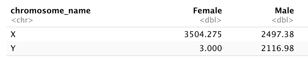
You will need to summarise before reshaping!
Let’s first calculate the mean expression level of X and Y linked genes from male and female samples…
R
 rna |>
  filter(chromosome_name == "Y" | chromosome_name == "X") |>
  group_by(sex, chromosome_name) |>
  summarise(mean = mean(expression))
OUTPUT
`summarise()` has regrouped the output.
ℹ Summaries were computed grouped by sex and chromosome_name.
ℹ Output is grouped by sex.
ℹ Use `summarise(.groups = "drop_last")` to silence this message.
ℹ Use `summarise(.by = c(sex, chromosome_name))` for per-operation grouping
  (`?dplyr::dplyr_by`) instead.
OUTPUT
# A tibble: 4 × 3
# Groups:   sex [2]
  sex    chromosome_name  mean
  <chr>  <chr>           <dbl>
1 Female X               3504.
2 Female Y                  3
3 Male   X               2497.
4 Male   Y               2117.
And pivot the table to wide format
R
rna_1 <- rna |>
  filter(chromosome_name == "Y" | chromosome_name == "X") |>
  group_by(sex, chromosome_name) |>
  summarise(mean = mean(expression)) |>
  pivot_wider(names_from = sex,
              values_from = mean)
OUTPUT
`summarise()` has regrouped the output.
ℹ Summaries were computed grouped by sex and chromosome_name.
ℹ Output is grouped by sex.
ℹ Use `summarise(.groups = "drop_last")` to silence this message.
ℹ Use `summarise(.by = c(sex, chromosome_name))` for per-operation grouping
  (`?dplyr::dplyr_by`) instead.
R
rna_1
OUTPUT
# A tibble: 2 × 3
  chromosome_name Female  Male
  <chr>            <dbl> <dbl>
1 X                3504. 2497.
2 Y                   3  2117.
Now take that data frame and transform it with
pivot_longer() so each row is a unique
chromosome_name by gender combination.
R
rna_1 |>
  pivot_longer(names_to = "gender",
               values_to = "mean",
               -chromosome_name)
OUTPUT
# A tibble: 4 × 3
  chromosome_name gender  mean
  <chr>           <chr>  <dbl>
1 X               Female 3504.
2 X               Male   2497.
3 Y               Female    3
4 Y Male 2117.Question
Use the rna dataset to create an expression matrix where
each row represents the mean expression levels of genes and columns
represent the different timepoints.
Let’s first calculate the mean expression by gene and by time
R
rna |>
  group_by(gene, time) |>
  summarise(mean_exp = mean(expression))
OUTPUT
`summarise()` has regrouped the output.
ℹ Summaries were computed grouped by gene and time.
ℹ Output is grouped by gene.
ℹ Use `summarise(.groups = "drop_last")` to silence this message.
ℹ Use `summarise(.by = c(gene, time))` for per-operation grouping
  (`?dplyr::dplyr_by`) instead.
OUTPUT
# A tibble: 4,422 × 3
# Groups:   gene [1,474]
   gene      time mean_exp
   <chr>    <dbl>    <dbl>
 1 AI504432     0    1034.
 2 AI504432     4    1104.
 3 AI504432     8    1014
 4 AW046200     0     155.
 5 AW046200     4     152.
 6 AW046200     8      81
 7 AW551984     0     238
 8 AW551984     4     302.
 9 AW551984     8     342.
10 Aamp         0    4603.
# ℹ 4,412 more rows
before using the pivot_wider() function
R
rna_time <- rna |>
  group_by(gene, time) |>
  summarise(mean_exp = mean(expression)) |>
  pivot_wider(names_from = time,
              values_from = mean_exp)
OUTPUT
`summarise()` has regrouped the output.
ℹ Summaries were computed grouped by gene and time.
ℹ Output is grouped by gene.
ℹ Use `summarise(.groups = "drop_last")` to silence this message.
ℹ Use `summarise(.by = c(gene, time))` for per-operation grouping
  (`?dplyr::dplyr_by`) instead.
R
rna_time
OUTPUT
# A tibble: 1,474 × 4
# Groups:   gene [1,474]
   gene         `0`     `4`     `8`
   <chr>      <dbl>   <dbl>   <dbl>
 1 AI504432 1034.   1104.   1014
 2 AW046200  155.    152.     81
 3 AW551984  238     302.    342.
 4 Aamp     4603.   4870    4763.
 5 Abca12      5.29    4.25    4.14
 6 Abcc8    2576.   2609.   2292.
 7 Abhd14a   591.    547.    432.
 8 Abi2     4881.   4903.   4945.
 9 Abi3bp   1175.   1061.    762.
10 Abl2     2170.   2078.   2131.
# ℹ 1,464 more rows
Notice that this generates a tibble with some column names starting by a number. If we wanted to select the column corresponding to the timepoints, we could not use the column names directly… What happens when we select the column 4?
R
rna |>
  group_by(gene, time) |>
  summarise(mean_exp = mean(expression)) |>
  pivot_wider(names_from = time,
              values_from = mean_exp) |>
  select(gene, 4)
OUTPUT
`summarise()` has regrouped the output.
ℹ Summaries were computed grouped by gene and time.
ℹ Output is grouped by gene.
ℹ Use `summarise(.groups = "drop_last")` to silence this message.
ℹ Use `summarise(.by = c(gene, time))` for per-operation grouping
  (`?dplyr::dplyr_by`) instead.
OUTPUT
# A tibble: 1,474 × 2
# Groups:   gene [1,474]
   gene         `8`
   <chr>      <dbl>
 1 AI504432 1014
 2 AW046200   81
 3 AW551984  342.
 4 Aamp     4763.
 5 Abca12      4.14
 6 Abcc8    2292.
 7 Abhd14a   432.
 8 Abi2     4945.
 9 Abi3bp    762.
10 Abl2     2131.
# ℹ 1,464 more rows
To select the timepoint 4, we would have to quote the column name, with backticks “`”
R
rna |>
  group_by(gene, time) |>
  summarise(mean_exp = mean(expression)) |>
  pivot_wider(names_from = time,
              values_from = mean_exp) |>
  select(gene, `4`)
OUTPUT
`summarise()` has regrouped the output.
ℹ Summaries were computed grouped by gene and time.
ℹ Output is grouped by gene.
ℹ Use `summarise(.groups = "drop_last")` to silence this message.
ℹ Use `summarise(.by = c(gene, time))` for per-operation grouping
  (`?dplyr::dplyr_by`) instead.
OUTPUT
# A tibble: 1,474 × 2
# Groups:   gene [1,474]
   gene         `4`
   <chr>      <dbl>
 1 AI504432 1104.
 2 AW046200  152.
 3 AW551984  302.
 4 Aamp     4870
 5 Abca12      4.25
 6 Abcc8    2609.
 7 Abhd14a   547.
 8 Abi2     4903.
 9 Abi3bp   1061.
10 Abl2     2078.
# ℹ 1,464 more rows
Another possibility would be to rename the column, choosing a name that doesn’t start by a number :
R
rna |>
  group_by(gene, time) |>
  summarise(mean_exp = mean(expression)) |>
  pivot_wider(names_from = time,
              values_from = mean_exp) |>
  rename("time0" = `0`, "time4" = `4`, "time8" = `8`) |>
  select(gene, time4)
OUTPUT
`summarise()` has regrouped the output.
ℹ Summaries were computed grouped by gene and time.
ℹ Output is grouped by gene.
ℹ Use `summarise(.groups = "drop_last")` to silence this message.
ℹ Use `summarise(.by = c(gene, time))` for per-operation grouping
  (`?dplyr::dplyr_by`) instead.
OUTPUT
# A tibble: 1,474 × 2
# Groups:   gene [1,474]
   gene       time4
   <chr>      <dbl>
 1 AI504432 1104.
 2 AW046200  152.
 3 AW551984  302.
 4 Aamp     4870
 5 Abca12      4.25
 6 Abcc8    2609.
 7 Abhd14a   547.
 8 Abi2     4903.
 9 Abi3bp   1061.
10 Abl2     2078.
# ℹ 1,464 more rowsQuestion
Use the previous data frame containing mean expression levels per timepoint and create a new column containing fold-changes between timepoint 8 and timepoint 0, and fold-changes between timepoint 8 and timepoint 4. Convert this table into a long-format table gathering the fold-changes calculated.
Starting from the rna_time tibble:
R
rna_time
OUTPUT
# A tibble: 1,474 × 4
# Groups:   gene [1,474]
   gene         `0`     `4`     `8`
   <chr>      <dbl>   <dbl>   <dbl>
 1 AI504432 1034.   1104.   1014
 2 AW046200  155.    152.     81
 3 AW551984  238     302.    342.
 4 Aamp     4603.   4870    4763.
 5 Abca12      5.29    4.25    4.14
 6 Abcc8    2576.   2609.   2292.
 7 Abhd14a   591.    547.    432.
 8 Abi2     4881.   4903.   4945.
 9 Abi3bp   1175.   1061.    762.
10 Abl2     2170.   2078.   2131.
# ℹ 1,464 more rows
Calculate fold-changes:
R
rna_time |>
  mutate(time_8_vs_0 = `8` / `0`, time_8_vs_4 = `8` / `4`)
OUTPUT
# A tibble: 1,474 × 6
# Groups:   gene [1,474]
   gene         `0`     `4`     `8` time_8_vs_0 time_8_vs_4
   <chr>      <dbl>   <dbl>   <dbl>       <dbl>       <dbl>
 1 AI504432 1034.   1104.   1014          0.981       0.918
 2 AW046200  155.    152.     81          0.522       0.532
 3 AW551984  238     302.    342.         1.44        1.13
 4 Aamp     4603.   4870    4763.         1.03        0.978
 5 Abca12      5.29    4.25    4.14       0.784       0.975
 6 Abcc8    2576.   2609.   2292.         0.889       0.878
 7 Abhd14a   591.    547.    432.         0.731       0.791
 8 Abi2     4881.   4903.   4945.         1.01        1.01
 9 Abi3bp   1175.   1061.    762.         0.649       0.719
10 Abl2     2170.   2078.   2131.         0.982       1.03
# ℹ 1,464 more rows
And use the pivot_longer() function:
R
rna_time |>
  mutate(time_8_vs_0 = `8` / `0`, time_8_vs_4 = `8` / `4`) |>
  pivot_longer(names_to = "comparisons",
               values_to = "Fold_changes",
               time_8_vs_0:time_8_vs_4)
OUTPUT
# A tibble: 2,948 × 6
# Groups:   gene [1,474]
   gene         `0`     `4`     `8` comparisons Fold_changes
   <chr>      <dbl>   <dbl>   <dbl> <chr>              <dbl>
 1 AI504432 1034.   1104.   1014    time_8_vs_0        0.981
 2 AI504432 1034.   1104.   1014    time_8_vs_4        0.918
 3 AW046200  155.    152.     81    time_8_vs_0        0.522
 4 AW046200  155.    152.     81    time_8_vs_4        0.532
 5 AW551984  238     302.    342.   time_8_vs_0        1.44
 6 AW551984  238     302.    342.   time_8_vs_4        1.13
 7 Aamp     4603.   4870    4763.   time_8_vs_0        1.03
 8 Aamp     4603.   4870    4763.   time_8_vs_4        0.978
 9 Abca12      5.29    4.25    4.14 time_8_vs_0        0.784
10 Abca12      5.29    4.25    4.14 time_8_vs_4        0.975
# ℹ 2,938 more rows
Joining tables
In many real life situations, data are spread across multiple tables. Usually this occurs because different types of information are collected from different sources.
It may be desirable for some analyses to combine data from two or more tables into a single data frame based on a column that would be common to all the tables.
The dplyr package provides a set of join functions for
combining two data frames based on matches within specified columns.
Here, we provide a short introduction to joins. For further reading,
please refer to the chapter about table
joins. The Data
Transformation Cheat Sheet also provides a short overview on table
joins.
We are going to illustrate join using a small table,
rna_mini that we will create by subsetting the original
rna table, keeping only 3 columns and 10 lines.
R
rna_mini <- rna |>
   select(gene, sample, expression) |>
   head(10)
rna_mini
OUTPUT
# A tibble: 10 × 3
   gene    sample     expression
   <chr>   <chr>           <dbl>
 1 Asl     GSM2545336       1170
 2 Apod    GSM2545336      36194
 3 Cyp2d22 GSM2545336       4060
 4 Klk6    GSM2545336        287
 5 Fcrls   GSM2545336         85
 6 Slc2a4  GSM2545336        782
 7 Exd2    GSM2545336       1619
 8 Gjc2    GSM2545336        288
 9 Plp1    GSM2545336      43217
10 Gnb4    GSM2545336       1071
The second table, annot1, contains 2 columns, gene and
gene_description. You can either download
annot1.csv by clicking on the link and then moving it to the
data/ folder, or you can use the R code below to download
it directly to the folder.
R
download.file(url = "https://carpentries-incubator.github.io/bioc-intro/data/annot1.csv",
              destfile = "data/annot1.csv")
annot1 <- read_csv(file = "data/annot1.csv")
annot1
OUTPUT
# A tibble: 10 × 2
gene gene_description
<chr> <chr>
1 Cyp2d22 cytochrome P450, family 2, subfamily d, polypeptide 22 [Source:MGI S…
2 Klk6 kallikrein related-peptidase 6 [Source:MGI Symbol;Acc:MGI:1343166]
3 Fcrls Fc receptor-like S, scavenger receptor [Source:MGI Symbol;Acc:MGI:19…
4 Plp1 proteolipid protein (myelin) 1 [Source:MGI Symbol;Acc:MGI:97623]
5 Exd2 exonuclease 3'-5' domain containing 2 [Source:MGI Symbol;Acc:MGI:192…
6 Apod apolipoprotein D [Source:MGI Symbol;Acc:MGI:88056]
7 Gnb4 guanine nucleotide binding protein (G protein), beta 4 [Source:MGI S…
8 Slc2a4 solute carrier family 2 (facilitated glucose transporter), member 4 …
9 Asl argininosuccinate lyase [Source:MGI Symbol;Acc:MGI:88084]
10 Gjc2 gap junction protein, gamma 2 [Source:MGI Symbol;Acc:MGI:2153060] We now want to join these two tables into a single one containing all
variables using the full_join() function from the
dplyr package. The function will automatically find the
common variable to match columns from the first and second table. In
this case, gene is the common variable. Such variables are
called keys. Keys are used to match observations across different
tables.
R
full_join(rna_mini, annot1)
OUTPUT
Joining with `by = join_by(gene)`OUTPUT
# A tibble: 10 × 4
gene sample expression gene_description
<chr> <chr> <dbl> <chr>
1 Asl GSM2545336 1170 argininosuccinate lyase [Source:MGI Symbol;Acc…
2 Apod GSM2545336 36194 apolipoprotein D [Source:MGI Symbol;Acc:MGI:88…
3 Cyp2d22 GSM2545336 4060 cytochrome P450, family 2, subfamily d, polype…
4 Klk6 GSM2545336 287 kallikrein related-peptidase 6 [Source:MGI Sym…
5 Fcrls GSM2545336 85 Fc receptor-like S, scavenger receptor [Source…
6 Slc2a4 GSM2545336 782 solute carrier family 2 (facilitated glucose t…
7 Exd2 GSM2545336 1619 exonuclease 3'-5' domain containing 2 [Source:…
8 Gjc2 GSM2545336 288 gap junction protein, gamma 2 [Source:MGI Symb…
9 Plp1 GSM2545336 43217 proteolipid protein (myelin) 1 [Source:MGI Sym…
10 Gnb4 GSM2545336 1071 guanine nucleotide binding protein (G protein)…In real life, gene annotations are sometimes labelled differently.
The annot2 table is exactly the same than
annot1 except that the variable containing gene names is
labelled differently. Again, either download
annot2.csv yourself and move it to data/ or use the R
code below.
R
download.file(url = "https://carpentries-incubator.github.io/bioc-intro/data/annot2.csv",
destfile = "data/annot2.csv")
annot2 <- read_csv(file = "data/annot2.csv")
annot2
OUTPUT
# A tibble: 10 × 2
external_gene_name description
<chr> <chr>
1 Cyp2d22 cytochrome P450, family 2, subfamily d, polypeptide 22 [S…
2 Klk6 kallikrein related-peptidase 6 [Source:MGI Symbol;Acc:MGI…
3 Fcrls Fc receptor-like S, scavenger receptor [Source:MGI Symbol…
4 Plp1 proteolipid protein (myelin) 1 [Source:MGI Symbol;Acc:MGI…
5 Exd2 exonuclease 3'-5' domain containing 2 [Source:MGI Symbol;…
6 Apod apolipoprotein D [Source:MGI Symbol;Acc:MGI:88056]
7 Gnb4 guanine nucleotide binding protein (G protein), beta 4 [S…
8 Slc2a4 solute carrier family 2 (facilitated glucose transporter)…
9 Asl argininosuccinate lyase [Source:MGI Symbol;Acc:MGI:88084]
10 Gjc2 gap junction protein, gamma 2 [Source:MGI Symbol;Acc:MGI:…In case none of the variable names match, we can set manually the
variables to use for the matching. These variables can be set using the
by argument, as shown below with rna_mini and
annot2 tables.
R
full_join(rna_mini, annot2, by = c("gene" = "external_gene_name"))
OUTPUT
# A tibble: 10 × 4
gene sample expression description
<chr> <chr> <dbl> <chr>
1 Asl GSM2545336 1170 argininosuccinate lyase [Source:MGI Symbol;Acc…
2 Apod GSM2545336 36194 apolipoprotein D [Source:MGI Symbol;Acc:MGI:88…
3 Cyp2d22 GSM2545336 4060 cytochrome P450, family 2, subfamily d, polype…
4 Klk6 GSM2545336 287 kallikrein related-peptidase 6 [Source:MGI Sym…
5 Fcrls GSM2545336 85 Fc receptor-like S, scavenger receptor [Source…
6 Slc2a4 GSM2545336 782 solute carrier family 2 (facilitated glucose t…
7 Exd2 GSM2545336 1619 exonuclease 3'-5' domain containing 2 [Source:…
8 Gjc2 GSM2545336 288 gap junction protein, gamma 2 [Source:MGI Symb…
9 Plp1 GSM2545336 43217 proteolipid protein (myelin) 1 [Source:MGI Sym…
10 Gnb4 GSM2545336 1071 guanine nucleotide binding protein (G protein)…As can be seen above, the variable name of the first table is retained in the joined one.
Challenge:
Download the annot3 table by clicking
this link and put the table in your data/ repository. Using the
full_join() function, join tables rna_mini and
annot3. What has happened for genes Klk6,
mt-Tf, mt-Rnr1, mt-Tv, mt-Rnr2, and
mt-Tl1 ?
R
annot3 <- read_csv("data/annot3.csv")
full_join(rna_mini, annot3)
OUTPUT
# A tibble: 15 × 4
gene sample expression gene_description
<chr> <chr> <dbl> <chr>
1 Asl GSM2545336 1170 argininosuccinate lyase [Source:MGI Symbol;Acc…
2 Apod GSM2545336 36194 apolipoprotein D [Source:MGI Symbol;Acc:MGI:88…
3 Cyp2d22 GSM2545336 4060 cytochrome P450, family 2, subfamily d, polype…
4 Klk6 GSM2545336 287 <NA>
5 Fcrls GSM2545336 85 Fc receptor-like S, scavenger receptor [Source…
6 Slc2a4 GSM2545336 782 solute carrier family 2 (facilitated glucose t…
7 Exd2 GSM2545336 1619 exonuclease 3'-5' domain containing 2 [Source:…
8 Gjc2 GSM2545336 288 gap junction protein, gamma 2 [Source:MGI Symb…
9 Plp1 GSM2545336 43217 proteolipid protein (myelin) 1 [Source:MGI Sym…
10 Gnb4 GSM2545336 1071 guanine nucleotide binding protein (G protein)…
11 mt-Tf <NA> NA mitochondrially encoded tRNA phenylalanine [So…
12 mt-Rnr1 <NA> NA mitochondrially encoded 12S rRNA [Source:MGI S…
13 mt-Tv <NA> NA mitochondrially encoded tRNA valine [Source:MG…
14 mt-Rnr2 <NA> NA mitochondrially encoded 16S rRNA [Source:MGI S…
15 mt-Tl1 <NA> NA mitochondrially encoded tRNA leucine 1 [Source…Genes Klk6 is only present in rna_mini, while
genes mt-Tf, mt-Rnr1, mt-Tv,
mt-Rnr2, and mt-Tl1 are only present in
annot3 table. Their respective values for the variables of
the table have been encoded as missing.
Exporting data
Now that you have learned how to use dplyr to extract
information from or summarise your raw data, you may want to export
these new data sets to share them with your collaborators or for
archival.
Similar to the read_csv() function used for reading CSV
files into R, there is a write_csv() function that
generates CSV files from data frames.
Before using write_csv(), we are going to create a new
folder, data_output, in our working directory that will
store this generated dataset. We don’t want to write generated datasets
in the same directory as our raw data. It’s good practice to keep them
separate. The data folder should only contain the raw,
unaltered data, and should be left alone to make sure we don’t delete or
modify it. In contrast, our script will generate the contents of the
data_output directory, so even if the files it contains are
deleted, we can always re-generate them.
Let’s use write_csv() to save the rna_wide table that we
have created previously.
R
write_csv(rna_wide, file = "data_output/rna_wide.csv")
- Tabular data in R using the tidyverse meta-package
Content from Data visualization
Last updated on 2026-07-14 | Edit this page
Overview
Questions
- Visualization in R
Objectives
- Produce scatter plots, boxplots, line plots, etc. using ggplot.
- Set universal plot settings.
- Describe what faceting is and apply faceting in ggplot.
- Modify the aesthetics of an existing ggplot plot (including axis labels and color).
- Build complex and customized plots from data in a data frame.
This episode is based on the Data Carpentries’s Data Analysis and Visualisation in R for Ecologists lesson.
Data Visualization
We start by loading the required packages.
ggplot2 is included in the
tidyverse package.
R
library("tidyverse")
If not still in the workspace, load the data we saved in the previous lesson.
R
rna <- read.csv("data/rnaseq.csv")
The Data
Visualization Cheat Sheet will cover the basics and more advanced
features of ggplot2 and will help, in addition to serve as
a reminder, getting an overview of the many data representations
available in the package. The following video tutorials (part 1 and part 2) by Thomas
Lin Pedersen are also very instructive.
Plotting with ggplot2
ggplot2 is a plotting package that makes it simple to
create complex plots from data in a data frame. It provides a more
programmatic interface for specifying what variables to plot, how they
are displayed, and general visual properties. The theoretical foundation
that supports the ggplot2 is the Grammar of
Graphics (@Wilkinson:2005). Using
this approach, we only need minimal changes if the underlying data
change or if we decide to change from a bar plot to a scatterplot. This
helps in creating publication quality plots with minimal amounts of
adjustments and tweaking.
There is a book about ggplot2 (@ggplot2book) that provides a good overview, but
it is outdated. The 3rd edition is in preparation and will be freely available online. The
ggplot2 webpage (https://ggplot2.tidyverse.org)
provides ample documentation.
ggplot2 functions like data in the ‘long’ format, i.e.,
a column for every dimension, and a row for every observation.
Well-structured data will save you lots of time when making figures with
ggplot2.
ggplot graphics are built step by step by adding new elements. Adding layers in this fashion allows for extensive flexibility and customization of plots.
The idea behind the Grammar of Graphics it is that you can build every graph from the same 3 components: (1) a data set, (2) a coordinate system, and (3) geoms — i.e. visual marks that represent data points 1
To build a ggplot, we will use the following basic template that can be used for different types of plots:
ggplot(data = <DATA>, mapping = aes(<MAPPINGS>)) + <GEOM_FUNCTION>()- use the
ggplot()function and bind the plot to a specific data frame using thedataargument
R
ggplot(data = rna)
- define a mapping (using the aesthetic
(
aes) function), by selecting the variables to be plotted and specifying how to present them in the graph, e.g. as x/y positions or characteristics such as size, shape, color, etc.
R
ggplot(data = rna, mapping = aes(x = expression))
-
add ‘geoms’ - geometries, or graphical representations of the data in the plot (points, lines, bars).
ggplot2offers many different geoms; we will use some common ones today, including:* `geom_point()` for scatter plots, dot plots, etc. * `geom_histogram()` for histograms * `geom_boxplot()` for, well, boxplots! * `geom_line()` for trend lines, time series, etc.
To add a geom(etry) to the plot use the + operator.
Let’s use geom_histogram() first:
R
ggplot(data = rna, mapping = aes(x = expression)) +
geom_histogram()
OUTPUT
`stat_bin()` using `bins = 30`. Pick better value `binwidth`.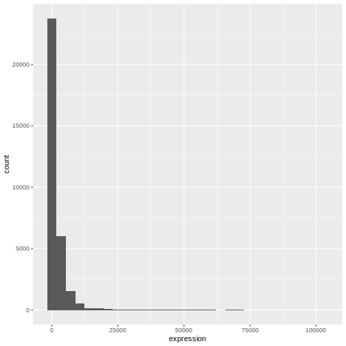
The + in the ggplot2 package is
particularly useful because it allows you to modify existing
ggplot objects. This means you can easily set up plot
templates and conveniently explore different types of plots, so the
above plot can also be generated with code like this:
R
# Assign plot to a variable
rna_plot <- ggplot(data = rna,
mapping = aes(x = expression))
# Draw the plot
rna_plot + geom_histogram()
Challenge
You have probably noticed an automatic message that appears when drawing the histogram:
OUTPUT
`stat_bin()` using `bins = 30`. Pick better value `binwidth`.Change the arguments bins or binwidth of
geom_histogram() to change the number or width of the
bins.
R
# change bins
ggplot(rna, aes(x = expression)) +
geom_histogram(bins = 15)
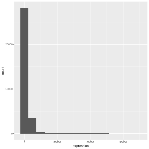
R
# change binwidth
ggplot(rna, aes(x = expression)) +
geom_histogram(binwidth = 2000)
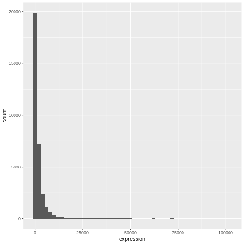
We can observe here that the data are skewed to the right. We can
apply log2 transformation to have a more symmetric distribution. Note
that we add here a small constant value (+1) to avoid
having -Inf values returned for expression values equal to
0.
R
rna <- rna |>
mutate(expression_log = log2(expression + 1))
If we now draw the histogram of the log2-transformed expressions, the distribution is indeed closer to a normal distribution.
R
ggplot(rna, aes(x = expression_log)) + geom_histogram()
OUTPUT
`stat_bin()` using `bins = 30`. Pick better value `binwidth`.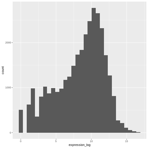
From now on we will work on the log-transformed expression values.
Challenge
Another way to visualize this transformation is to consider the scale of the observations. For example, it may be worth changing the scale of the axis to better distribute the observations in the space of the plot. Changing the scale of the axes is done similarly to adding/modifying other components (i.e., by incrementally adding commands). Try making this modification:
- Represent the un-transformed expression on the log10 scale; see
scale_x_log10(). Compare it with the previous graph. Why do you now have warning messages appearing?
R
ggplot(data = rna,mapping = aes(x = expression))+
geom_histogram() +
scale_x_log10()
WARNING
Warning in scale_x_log10(): log-10 transformation introduced infinite values.OUTPUT
`stat_bin()` using `bins = 30`. Pick better value `binwidth`.WARNING
Warning: Removed 507 rows containing non-finite outside the scale range
(`stat_bin()`).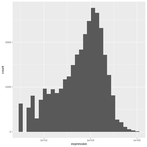
Notes
- Anything you put in the
ggplot()function can be seen by any geom layers that you add (i.e., these are global plot settings). This includes the x- and y-axis mapping you set up inaes(). - You can also specify mappings for a given geom independently of the
mappings defined globally in the
ggplot()function. - The
+sign used to add new layers must be placed at the end of the line containing the previous layer. If, instead, the+sign is added at the beginning of the line containing the new layer,ggplot2will not add the new layer and will return an error message.
R
# This is the correct syntax for adding layers
rna_plot +
geom_histogram()
# This will not add the new layer and will return an error message
rna_plot
+ geom_histogram()
Building your plots iteratively
We will now draw a scatter plot with two continuous variables and the
geom_point() function. This graph will represent the log2
fold changes of expression comparing time 8 versus time 0, and time 4
versus time 0. To this end, we first need to compute the means of the
log-transformed expression values by gene and time, then the log fold
changes by subtracting the mean log expressions between time 8 and time
0 and between time 4 and time 0. Note that we also include here the gene
biotype that we will use later on to represent the genes. We will save
the fold changes in a new data frame called rna_fc.
R
rna_fc <- rna |> select(gene, time,
gene_biotype, expression_log) |>
group_by(gene, time, gene_biotype) |>
summarize(mean_exp = mean(expression_log)) |>
pivot_wider(names_from = time,
values_from = mean_exp) |>
mutate(time_8_vs_0 = `8` - `0`, time_4_vs_0 = `4` - `0`)
OUTPUT
`summarise()` has regrouped the output.
ℹ Summaries were computed grouped by gene, time, and gene_biotype.
ℹ Output is grouped by gene and time.
ℹ Use `summarise(.groups = "drop_last")` to silence this message.
ℹ Use `summarise(.by = c(gene, time, gene_biotype))` for per-operation grouping
(`?dplyr::dplyr_by`) instead.We can then build a ggplot with the newly created dataset
rna_fc. Building plots with ggplot2 is
typically an iterative process. We start by defining the dataset we’ll
use, lay out the axes, and choose a geom:
R
ggplot(data = rna_fc, mapping = aes(x = time_4_vs_0, y = time_8_vs_0)) +
geom_point()
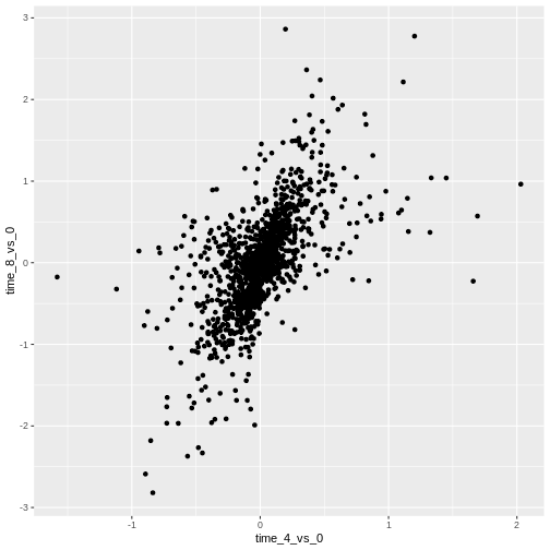
Then, we start modifying this plot to extract more information from
it. For instance, we can add transparency (alpha) to avoid
overplotting:
R
ggplot(data = rna_fc, mapping = aes(x = time_4_vs_0, y = time_8_vs_0)) +
geom_point(alpha = 0.3)
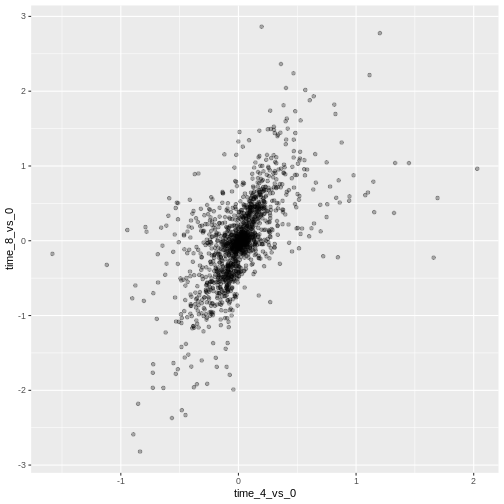
We can also add colors for all the points:
R
ggplot(data = rna_fc, mapping = aes(x = time_4_vs_0, y = time_8_vs_0)) +
geom_point(alpha = 0.3, color = "blue")
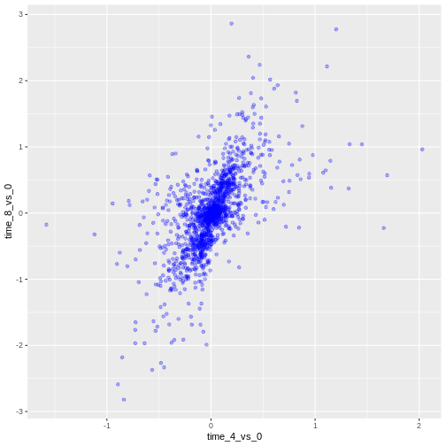
Or to color each gene in the plot differently, you could use a vector
as an input to the argument color. ggplot2
will provide a different color corresponding to different values in the
vector. Here is an example where we color with
gene_biotype:
R
ggplot(data = rna_fc, mapping = aes(x = time_4_vs_0, y = time_8_vs_0)) +
geom_point(alpha = 0.3, aes(color = gene_biotype))
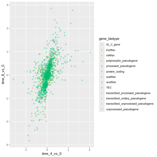
We can also specify the colors directly inside the mapping provided
in the ggplot() function. This will be seen by any geom
layers and the mapping will be determined by the x- and y-axis set up in
aes().
R
ggplot(data = rna_fc, mapping = aes(x = time_4_vs_0, y = time_8_vs_0,
color = gene_biotype)) +
geom_point(alpha = 0.3)

Finally, we could also add a diagonal line with the
geom_abline() function:
R
ggplot(data = rna_fc, mapping = aes(x = time_4_vs_0, y = time_8_vs_0,
color = gene_biotype)) +
geom_point(alpha = 0.3) +
geom_abline(intercept = 0)

Notice that we can change the geom layer from geom_point
to geom_jitter and colors will still be determined by
gene_biotype.
R
ggplot(data = rna_fc, mapping = aes(x = time_4_vs_0, y = time_8_vs_0,
color = gene_biotype)) +
geom_jitter(alpha = 0.3) +
geom_abline(intercept = 0)
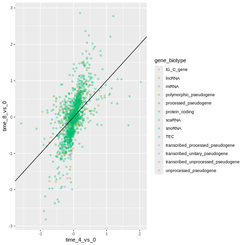
Challenge
Scatter plots can be useful exploratory tools for small datasets. For
data sets with large numbers of observations, such as the
rna_fc data set, overplotting of points can be a limitation
of scatter plots. One strategy for handling such settings is to use
hexagonal binning of observations. The plot space is tessellated into
hexagons. Each hexagon is assigned a color based on the number of
observations that fall within its boundaries.
To use hexagonal binning in
ggplot2, first install the R packagehexbinfrom CRAN and load it.Then use the
geom_hex()function to produce the hexbin figure.What are the relative strengths and weaknesses of a hexagonal bin plot compared to a scatter plot? Examine the above scatter plot and compare it with the hexagonal bin plot that you created.
R
install.packages("hexbin")
R
library("hexbin")
ggplot(data = rna_fc, mapping = aes(x = time_4_vs_0, y = time_8_vs_0)) +
geom_hex() +
geom_abline(intercept = 0)
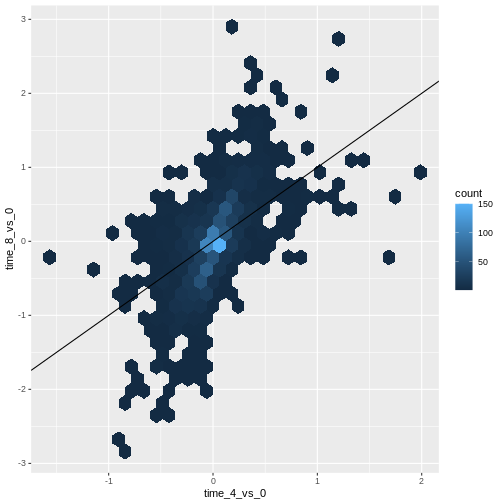
Challenge
Use what you just learned to create a scatter plot of
expression_log over sample from the
rna dataset with the time showing in different colors. Is
this a good way to show this type of data?
R
ggplot(data = rna, mapping = aes(y = expression_log, x = sample)) +
geom_point(aes(color = time))
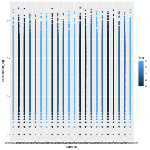
Boxplot
We can use boxplots to visualize the distribution of gene expressions within each sample:
R
ggplot(data = rna,
mapping = aes(y = expression_log, x = sample)) +
geom_boxplot()
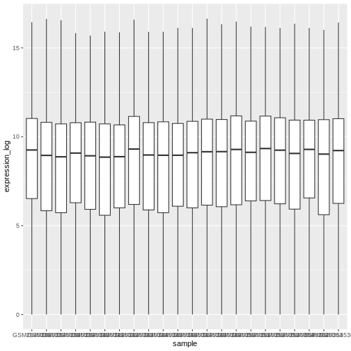
By adding points to boxplot, we can have a better idea of the number of measurements and of their distribution:
R
ggplot(data = rna,
mapping = aes(y = expression_log, x = sample)) +
geom_jitter(alpha = 0.2, color = "tomato") +
geom_boxplot(alpha = 0)
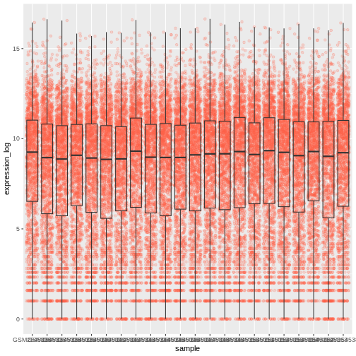
Challenge
Note how the boxplot layer is in front of the jitter layer? What do you need to change in the code to put the boxplot below the points?
We should switch the order of these two geoms:
R
ggplot(data = rna,
mapping = aes(y = expression_log, x = sample)) +
geom_boxplot(alpha = 0) +
geom_jitter(alpha = 0.2, color = "tomato")
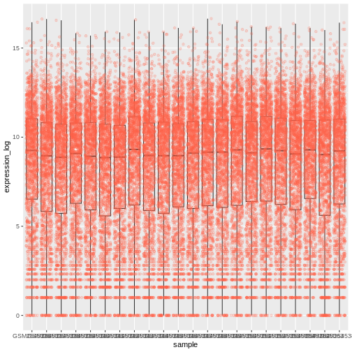
You may notice that the values on the x-axis are still not properly readable. Let’s change the orientation of the labels and adjust them vertically and horizontally so they don’t overlap. You can use a 90-degree angle, or experiment to find the appropriate angle for diagonally oriented labels:
R
ggplot(data = rna,
mapping = aes(y = expression_log, x = sample)) +
geom_jitter(alpha = 0.2, color = "tomato") +
geom_boxplot(alpha = 0) +
theme(axis.text.x = element_text(angle = 90, hjust = 0.5, vjust = 0.5))
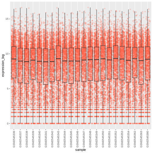
Challenge
Add color to the data points on your boxplot according to the
duration of the infection (time).
Hint: Check the class for time. Consider
changing the class of time from integer to factor directly
in the ggplot mapping. Why does this change how R makes the graph?
R
# time as integer
ggplot(data = rna,
mapping = aes(y = expression_log,
x = sample)) +
geom_jitter(alpha = 0.2, aes(color = time)) +
geom_boxplot(alpha = 0) +
theme(axis.text.x = element_text(angle = 90, hjust = 0.5, vjust = 0.5))
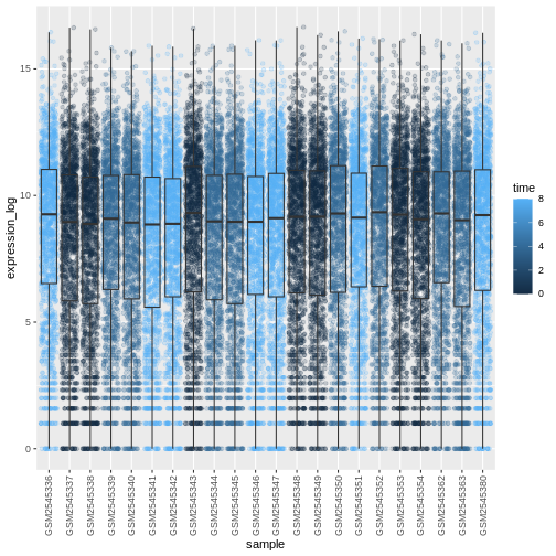
R
# time as factor
ggplot(data = rna,
mapping = aes(y = expression_log,
x = sample)) +
geom_jitter(alpha = 0.2, aes(color = as.factor(time))) +
geom_boxplot(alpha = 0) +
theme(axis.text.x = element_text(angle = 90, hjust = 0.5, vjust = 0.5))
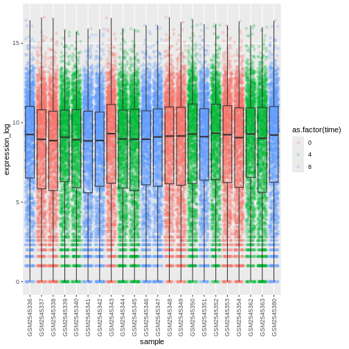
Challenge
Boxplots are useful summaries, but hide the shape of the distribution. For example, if the distribution is bimodal, we would not see it in a boxplot. An alternative to the boxplot is the violin plot, where the shape (of the density of points) is drawn.
- Replace the box plot with a violin plot; see
geom_violin(). Fill in the violins according to the time with the argumentfill.
R
ggplot(data = rna,
mapping = aes(y = expression_log, x = sample)) +
geom_violin(aes(fill = as.factor(time))) +
theme(axis.text.x = element_text(angle = 90, hjust = 0.5, vjust = 0.5))
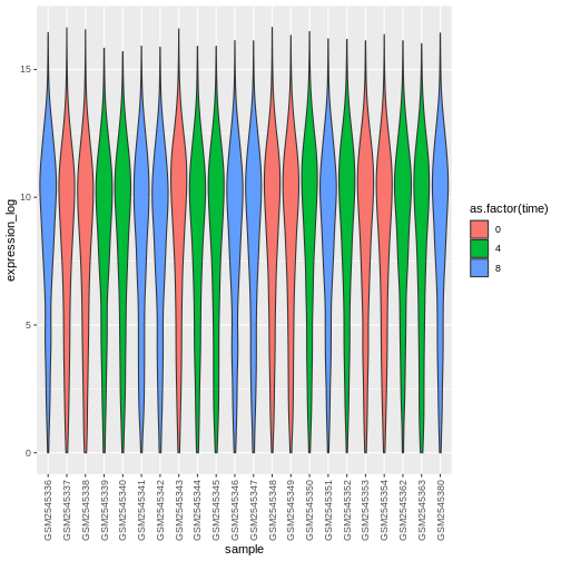
Challenge
- Modify the violin plot to fill in the violins by
sex.
R
ggplot(data = rna,
mapping = aes(y = expression_log, x = sample)) +
geom_violin(aes(fill = sex)) +
theme(axis.text.x = element_text(angle = 90, hjust = 0.5, vjust = 0.5))
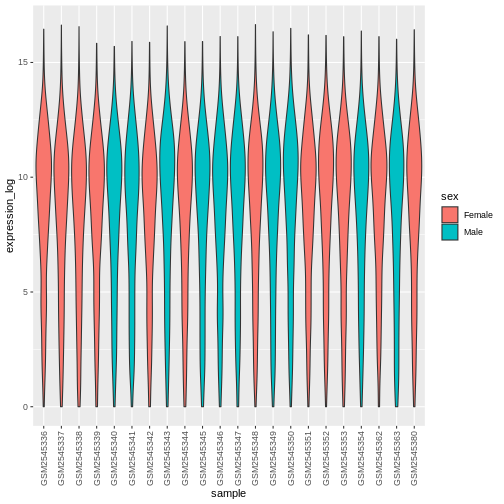
Line plots
Let’s calculate the mean expression per duration of the infection for
the 10 genes having the highest log fold changes comparing time 8 versus
time 0. First, we need to select the genes and create a subset of
rna called sub_rna containing the 10 selected
genes, then we need to group the data and calculate the mean gene
expression within each group:
R
rna_fc <- rna_fc |> arrange(desc(time_8_vs_0))
genes_selected <- rna_fc$gene[1:10]
sub_rna <- rna |>
filter(gene %in% genes_selected)
mean_exp_by_time <- sub_rna |>
group_by(gene,time) |>
summarize(mean_exp = mean(expression_log))
OUTPUT
`summarise()` has regrouped the output.
ℹ Summaries were computed grouped by gene and time.
ℹ Output is grouped by gene.
ℹ Use `summarise(.groups = "drop_last")` to silence this message.
ℹ Use `summarise(.by = c(gene, time))` for per-operation grouping
(`?dplyr::dplyr_by`) instead.R
mean_exp_by_time
OUTPUT
# A tibble: 30 × 3
# Groups: gene [10]
gene time mean_exp
<chr> <int> <dbl>
1 Acr 0 5.07
2 Acr 4 5.54
3 Acr 8 7.31
4 Aipl1 0 3.70
5 Aipl1 4 3.89
6 Aipl1 8 6.56
7 Bst1 0 3.20
8 Bst1 4 3.77
9 Bst1 8 5.22
10 Chil3 0 4.00
# ℹ 20 more rowsWe can build the line plot with duration of the infection on the x-axis and the mean expression on the y-axis:
R
ggplot(data = mean_exp_by_time, mapping = aes(x = time, y = mean_exp)) +
geom_line()
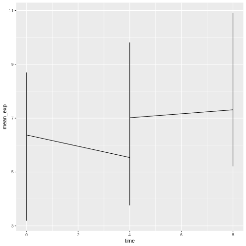
Unfortunately, this does not work because we plotted data for all the
genes together. We need to tell ggplot to draw a line for each gene by
modifying the aesthetic function to include
group = gene:
R
ggplot(data = mean_exp_by_time,
mapping = aes(x = time, y = mean_exp, group = gene)) +
geom_line()
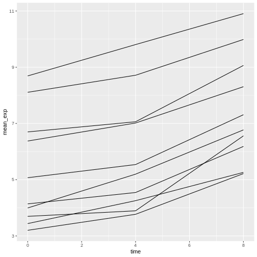
We will be able to distinguish genes in the plot if we add colors
(using color also automatically groups the data):
R
ggplot(data = mean_exp_by_time,
mapping = aes(x = time, y = mean_exp, color = gene)) +
geom_line()
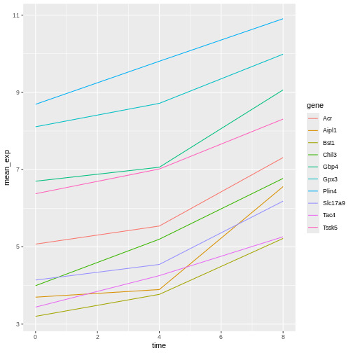
Faceting
ggplot2 has a special technique called faceting
that allows the user to split one plot into multiple (sub) plots based
on a factor included in the dataset. These different subplots inherit
the same properties (axes limits, ticks, …) to facilitate their direct
comparison. We will use it to make a line plot across time for each
gene:
R
ggplot(data = mean_exp_by_time,
mapping = aes(x = time, y = mean_exp)) + geom_line() +
facet_wrap(~ gene)
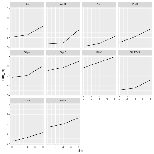
Here both x- and y-axis have the same scale for all the subplots. You
can change this default behavior by modifying scales in
order to allow a free scale for the y-axis:
R
ggplot(data = mean_exp_by_time,
mapping = aes(x = time, y = mean_exp)) +
geom_line() +
facet_wrap(~ gene, scales = "free_y")
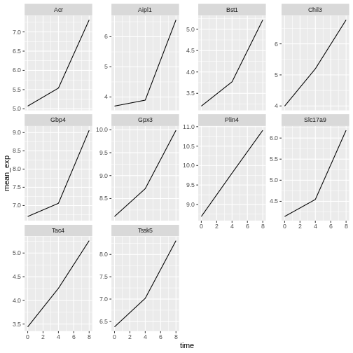
Now we would like to split the line in each plot by the sex of the
mice. To do that we need to calculate the mean expression in the data
frame grouped by gene, time, and
sex:
R
mean_exp_by_time_sex <- sub_rna |>
group_by(gene, time, sex) |>
summarize(mean_exp = mean(expression_log))
OUTPUT
`summarise()` has regrouped the output.
ℹ Summaries were computed grouped by gene, time, and sex.
ℹ Output is grouped by gene and time.
ℹ Use `summarise(.groups = "drop_last")` to silence this message.
ℹ Use `summarise(.by = c(gene, time, sex))` for per-operation grouping
(`?dplyr::dplyr_by`) instead.R
mean_exp_by_time_sex
OUTPUT
# A tibble: 60 × 4
# Groups: gene, time [30]
gene time sex mean_exp
<chr> <int> <chr> <dbl>
1 Acr 0 Female 5.13
2 Acr 0 Male 5.00
3 Acr 4 Female 5.93
4 Acr 4 Male 5.15
5 Acr 8 Female 7.27
6 Acr 8 Male 7.36
7 Aipl1 0 Female 3.67
8 Aipl1 0 Male 3.73
9 Aipl1 4 Female 4.07
10 Aipl1 4 Male 3.72
# ℹ 50 more rowsWe can now make the faceted plot by splitting further by sex using
color (within a single plot):
R
ggplot(data = mean_exp_by_time_sex,
mapping = aes(x = time, y = mean_exp, color = sex)) +
geom_line() +
facet_wrap(~ gene, scales = "free_y")
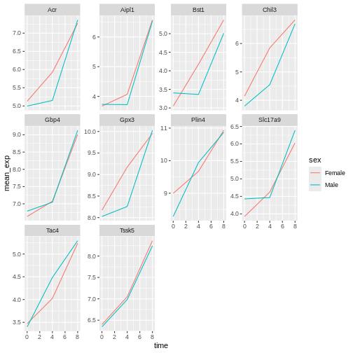
Usually plots with white background look more readable when printed.
We can set the background to white using the function
theme_bw(). Additionally, we can remove the grid:
R
ggplot(data = mean_exp_by_time_sex,
mapping = aes(x = time, y = mean_exp, color = sex)) +
geom_line() +
facet_wrap(~ gene, scales = "free_y") +
theme_bw() +
theme(panel.grid = element_blank())
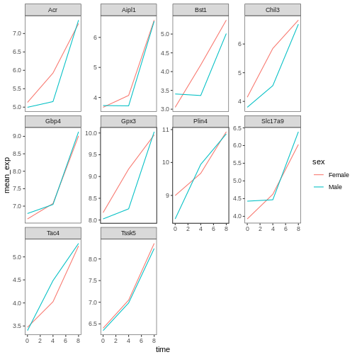
Challenge
Use what you just learned to create a plot that depicts how the average expression of each chromosome changes through the duration of infection.
R
mean_exp_by_chromosome <- rna |>
group_by(chromosome_name, time) |>
summarize(mean_exp = mean(expression_log))
OUTPUT
`summarise()` has regrouped the output.
ℹ Summaries were computed grouped by chromosome_name and time.
ℹ Output is grouped by chromosome_name.
ℹ Use `summarise(.groups = "drop_last")` to silence this message.
ℹ Use `summarise(.by = c(chromosome_name, time))` for per-operation grouping
(`?dplyr::dplyr_by`) instead.R
ggplot(data = mean_exp_by_chromosome, mapping = aes(x = time,
y = mean_exp)) +
geom_line() +
facet_wrap(~ chromosome_name, scales = "free_y")
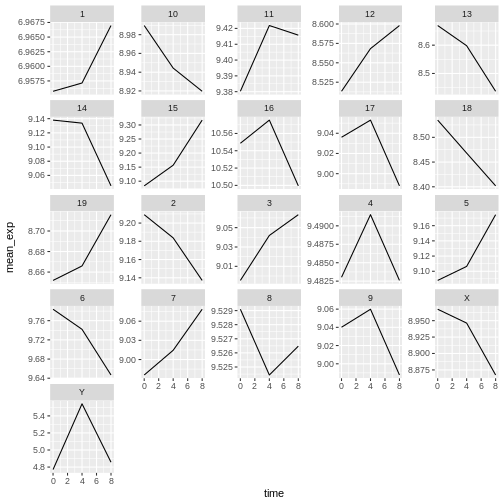
The facet_wrap geometry extracts plots into an arbitrary
number of dimensions to allow them to cleanly fit on one page. On the
other hand, the facet_grid geometry allows you to
explicitly specify how you want your plots to be arranged via formula
notation (rows ~ columns; a . can be used as a
placeholder that indicates only one row or column).
Let’s modify the previous plot to compare how the mean gene expression of males and females has changed through time:
R
# One column, facet by rows
ggplot(data = mean_exp_by_time_sex,
mapping = aes(x = time, y = mean_exp, color = gene)) +
geom_line() +
facet_grid(sex ~ .)
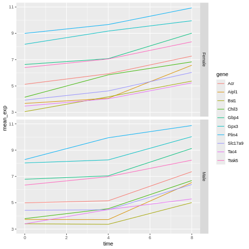
R
# One row, facet by column
ggplot(data = mean_exp_by_time_sex,
mapping = aes(x = time, y = mean_exp, color = gene)) +
geom_line() +
facet_grid(. ~ sex)
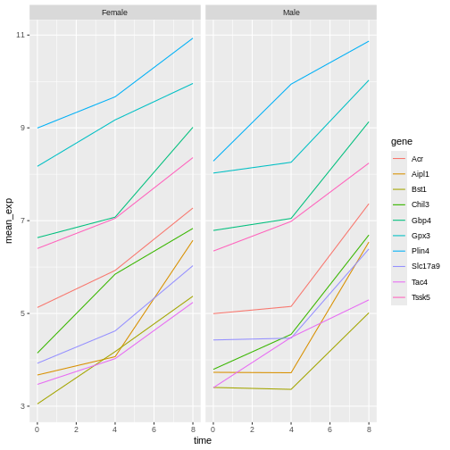
ggplot2 themes
In addition to theme_bw(), which changes the plot
background to white, ggplot2 comes with several other
themes which can be useful to quickly change the look of your
visualization. The complete list of themes is available at https://ggplot2.tidyverse.org/reference/ggtheme.html.
theme_minimal() and theme_light() are popular,
and theme_void() can be useful as a starting point to
create a new hand-crafted theme.
The ggthemes
package provides a wide variety of options (including an Excel 2003
theme). The ggplot2
extensions website provides a list of packages that extend the
capabilities of ggplot2, including additional themes.
Customisation
Let’s come back to the faceted plot of mean expression by time and gene, colored by sex.
Take a look at the ggplot2
cheat sheet, and think of ways you could improve the plot.
Now, we can change names of axes to something more informative than ‘time’ and ‘mean_exp’, and add a title to the figure:
R
ggplot(data = mean_exp_by_time_sex,
mapping = aes(x = time, y = mean_exp, color = sex)) +
geom_line() +
facet_wrap(~ gene, scales = "free_y") +
theme_bw() +
theme(panel.grid = element_blank()) +
labs(title = "Mean gene expression by duration of the infection",
x = "Duration of the infection (in days)",
y = "Mean gene expression")
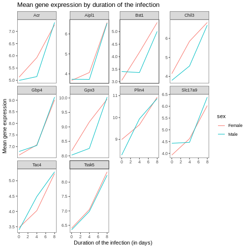
The axes have more informative names, but their readability can be improved by increasing the font size:
R
ggplot(data = mean_exp_by_time_sex,
mapping = aes(x = time, y = mean_exp, color = sex)) +
geom_line() +
facet_wrap(~ gene, scales = "free_y") +
theme_bw() +
theme(panel.grid = element_blank()) +
labs(title = "Mean gene expression by duration of the infection",
x = "Duration of the infection (in days)",
y = "Mean gene expression") +
theme(text = element_text(size = 16))
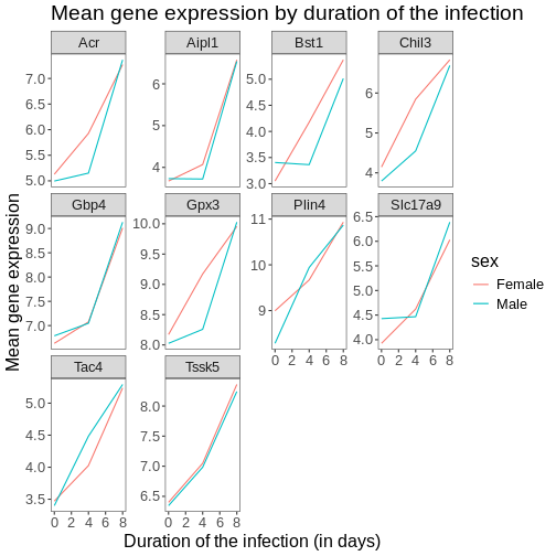
Note that it is also possible to change the fonts of your plots. If
you are on Windows, you may have to install the extrafont
package.
We can further customize the color of x- and y-axis text, the color
of the grid, etc. We can also for example move the legend to the top by
setting legend.position to "top".
R
ggplot(data = mean_exp_by_time_sex,
mapping = aes(x = time, y = mean_exp, color = sex)) +
geom_line() +
facet_wrap(~ gene, scales = "free_y") +
theme_bw() +
theme(panel.grid = element_blank()) +
labs(title = "Mean gene expression by duration of the infection",
x = "Duration of the infection (in days)",
y = "Mean gene expression") +
theme(text = element_text(size = 16),
axis.text.x = element_text(colour = "royalblue4", size = 12),
axis.text.y = element_text(colour = "royalblue4", size = 12),
panel.grid = element_line(colour="lightsteelblue1"),
legend.position = "top")
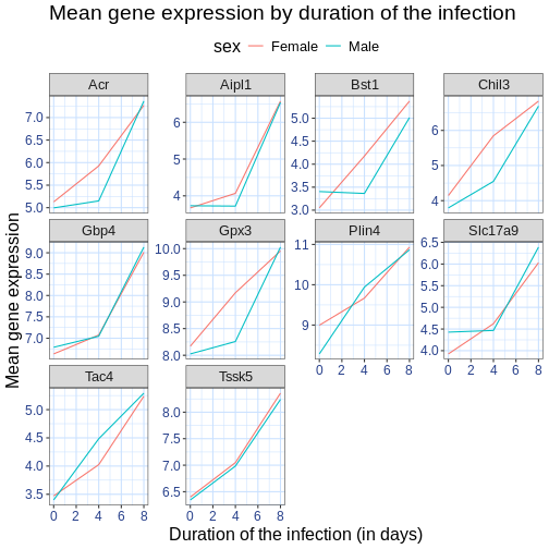
If you like the changes you created better than the default theme, you can save them as an object to be able to easily apply them to other plots you may create. Here is an example with the histogram we have previously created.
R
blue_theme <- theme(axis.text.x = element_text(colour = "royalblue4",
size = 12),
axis.text.y = element_text(colour = "royalblue4",
size = 12),
text = element_text(size = 16),
panel.grid = element_line(colour="lightsteelblue1"))
ggplot(rna, aes(x = expression_log)) +
geom_histogram(bins = 20) +
blue_theme()
ERROR
Error in `blue_theme()`:
! could not find function "blue_theme"Challenge
With all of this information in hand, please take another five
minutes to either improve one of the plots generated in this exercise or
create a beautiful graph of your own. Use the RStudio ggplot2
cheat sheet for inspiration. Here are some ideas:
- See if you can change the thickness of the lines.
- Can you find a way to change the name of the legend? What about its
labels? (hint: look for a ggplot function starting with
scale_) - Try using a different color palette or manually specifying the colors for the lines (see https://www.cookbook-r.com/Graphs/Colors_(ggplot2)/).
For example, based on this plot:
R
ggplot(data = mean_exp_by_time_sex,
mapping = aes(x = time, y = mean_exp, color = sex)) +
geom_line() +
facet_wrap(~ gene, scales = "free_y") +
theme_bw() +
theme(panel.grid = element_blank())

We can customize it the following ways:
R
# change the thickness of the lines
ggplot(data = mean_exp_by_time_sex,
mapping = aes(x = time, y = mean_exp, color = sex)) +
geom_line(size=1.5) +
facet_wrap(~ gene, scales = "free_y") +
theme_bw() +
theme(panel.grid = element_blank())
WARNING
Warning: Using `size` aesthetic for lines was deprecated in ggplot2 3.4.0.
ℹ Please use `linewidth` instead.
This warning is displayed once per session.
Call `lifecycle::last_lifecycle_warnings()` to see where this warning was
generated.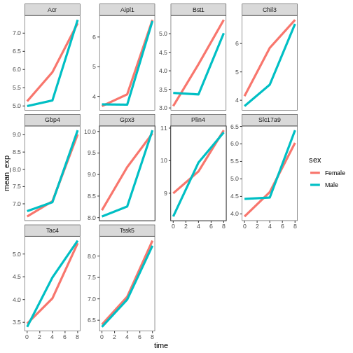
R
# change the name of the legend and the labels
ggplot(data = mean_exp_by_time_sex,
mapping = aes(x = time, y = mean_exp, color = sex)) +
geom_line() +
facet_wrap(~ gene, scales = "free_y") +
theme_bw() +
theme(panel.grid = element_blank()) +
scale_color_discrete(name = "Gender", labels = c("F", "M"))
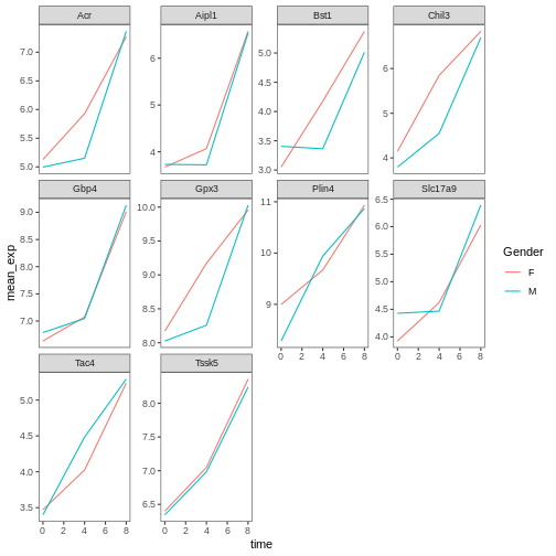
R
# using a different color palette
ggplot(data = mean_exp_by_time_sex,
mapping = aes(x = time, y = mean_exp, color = sex)) +
geom_line() +
facet_wrap(~ gene, scales = "free_y") +
theme_bw() +
theme(panel.grid = element_blank()) +
scale_color_brewer(name = "Gender", labels = c("F", "M"), palette = "Dark2")
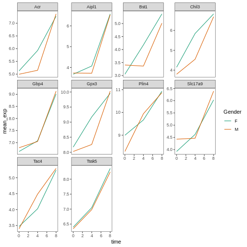
R
# manually specifying the colors
ggplot(data = mean_exp_by_time_sex,
mapping = aes(x = time, y = mean_exp, color = sex)) +
geom_line() +
facet_wrap(~ gene, scales = "free_y") +
theme_bw() +
theme(panel.grid = element_blank()) +
scale_color_manual(name = "Gender", labels = c("F", "M"),
values = c("royalblue", "deeppink"))
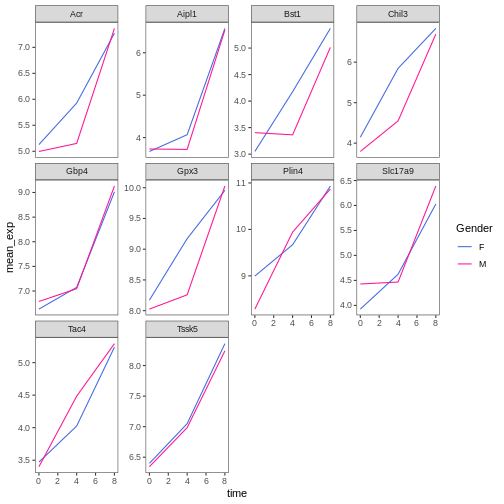
Composing plots
Faceting is a great tool for splitting one plot into multiple subplots, but sometimes you may want to produce a single figure that contains multiple independent plots, i.e. plots that are based on different variables or even different data frames.
Let’s start by creating the two plots that we want to arrange next to each other:
The first graph counts the number of unique genes per chromosome. We
first need to reorder the levels of chromosome_name and
filter the unique genes per chromosome. We also change the scale of the
y-axis to a log10 scale for better readability.
R
rna$chromosome_name <- factor(rna$chromosome_name,
levels = c(1:19,"X","Y"))
count_gene_chromosome <- rna |>
select(chromosome_name, gene) |>
distinct() |> ggplot() +
geom_bar(aes(x = chromosome_name), fill = "seagreen",
position = "dodge", stat = "count") +
labs(y = "log10(n genes)", x = "chromosome") +
scale_y_log10()
count_gene_chromosome
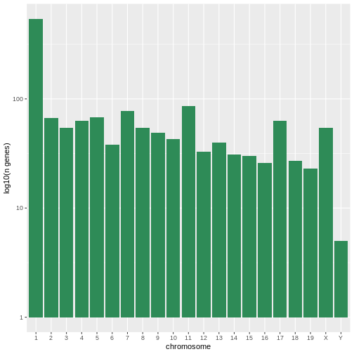
Below, we also remove the legend altogether by setting the
legend.position to "none".
R
exp_boxplot_sex <- ggplot(rna, aes(y=expression_log, x = as.factor(time),
color=sex)) +
geom_boxplot(alpha = 0) +
labs(y = "Mean gene exp",
x = "time") + theme(legend.position = "none")
exp_boxplot_sex
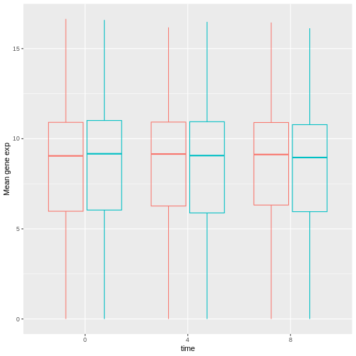
The patchwork
package provides an elegant approach to combining figures using the
+ to arrange figures (typically side by side). More
specifically the | explicitly arranges them side by side
and / stacks them on top of each other.
R
install.packages("patchwork")
R
library("patchwork")
count_gene_chromosome + exp_boxplot_sex
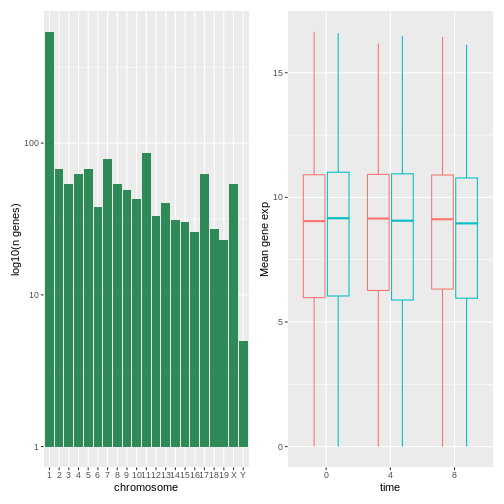
R
## or count_gene_chromosome | exp_boxplot_sex
R
count_gene_chromosome / exp_boxplot_sex
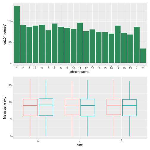
We can combine further control the layout of the final composition
with plot_layout to create more complex layouts:
R
count_gene_chromosome + exp_boxplot_sex + plot_layout(ncol = 1)

R
count_gene_chromosome +
(count_gene_chromosome + exp_boxplot_sex) +
exp_boxplot_sex +
plot_layout(ncol = 1)

The last plot can also be created using the | and
/ composers:
R
count_gene_chromosome /
(count_gene_chromosome | exp_boxplot_sex) /
exp_boxplot_sex
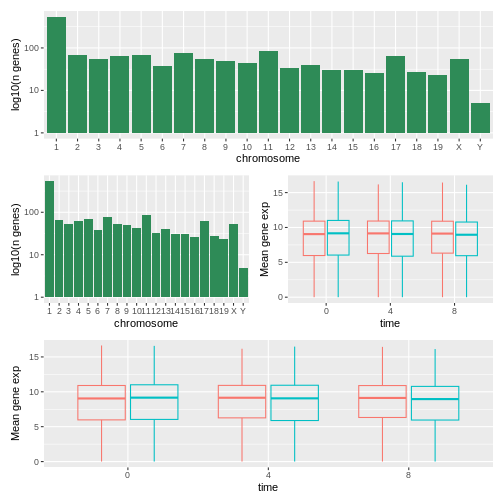
Learn more about patchwork on its webpage or in this video.
Another option is the gridExtra package
that allows to combine separate ggplots into a single figure using
grid.arrange():
R
install.packages("gridExtra")
R
library("gridExtra")
grid.arrange(count_gene_chromosome, exp_boxplot_sex, ncol = 2)
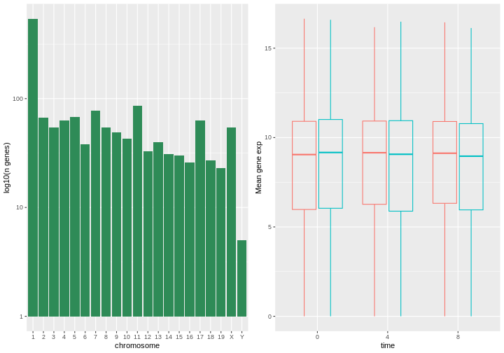
In addition to the ncol and nrow arguments,
used to make simple arrangements, there are tools for constructing
more complex layouts.
Exporting plots
After creating your plot, you can save it to a file in your favorite format. The Export tab in the Plot pane in RStudio will save your plots at low resolution, which will not be accepted by many journals and will not scale well for posters.
Instead, use the ggsave() function, which allows you
easily change the dimension and resolution of your plot by adjusting the
appropriate arguments (width, height and
dpi).
Make sure you have the fig_output/ folder in your
working directory.
R
my_plot <- ggplot(data = mean_exp_by_time_sex,
mapping = aes(x = time, y = mean_exp, color = sex)) +
geom_line() +
facet_wrap(~ gene, scales = "free_y") +
labs(title = "Mean gene expression by duration of the infection",
x = "Duration of the infection (in days)",
y = "Mean gene expression") +
guides(color=guide_legend(title="Gender")) +
theme_bw() +
theme(axis.text.x = element_text(colour = "royalblue4", size = 12),
axis.text.y = element_text(colour = "royalblue4", size = 12),
text = element_text(size = 16),
panel.grid = element_line(colour="lightsteelblue1"),
legend.position = "top")
ggsave("fig_output/mean_exp_by_time_sex.png", my_plot, width = 15,
height = 10)
# This also works for grid.arrange() plots
combo_plot <- grid.arrange(count_gene_chromosome, exp_boxplot_sex,
ncol = 2, widths = c(4, 6))
ggsave("fig_output/combo_plot_chromosome_sex.png", combo_plot,
width = 10, dpi = 300)
Note: The parameters width and height also
determine the font size in the saved plot.
Other packages for visualisation
ggplot2 is a very powerful package that fits very nicely
in our tidy data and tidy tools pipeline. There are
other visualization packages in R that shouldn’t be ignored.
Base graphics
The default graphics system that comes with R, often called base
R graphics is simple and fast. It is based on the painter’s or
canvas model, where different output are directly overlaid on top
of each other (see figure @ref(fig:paintermodel)). This is a fundamental
difference with ggplot2 (and with lattice,
described below), that returns dedicated objects, that are rendered on
screen or in a file, and that can even be updated.
R
par(mfrow = c(1, 3))
plot(1:20, main = "First layer, produced with plot(1:20)")
plot(1:20, main = "A horizontal red line, added with abline(h = 10)")
abline(h = 10, col = "red")
plot(1:20, main = "A rectangle, added with rect(5, 5, 15, 15)")
abline(h = 10, col = "red")
rect(5, 5, 15, 15, lwd = 3)
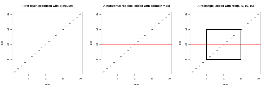
Another main difference is that base graphics’ plotting function try
to do the right thing based on their input type, i.e. they will
adapt their behaviour based on the class of their input. This is again
very different from what we have in ggplot2, that only
accepts dataframes as input, and that requires plots to be constructed
bit by bit.
R
par(mfrow = c(2, 2))
boxplot(rnorm(100),
main = "Boxplot of rnorm(100)")
boxplot(matrix(rnorm(100), ncol = 10),
main = "Boxplot of matrix(rnorm(100), ncol = 10)")
hist(rnorm(100))
hist(matrix(rnorm(100), ncol = 10))
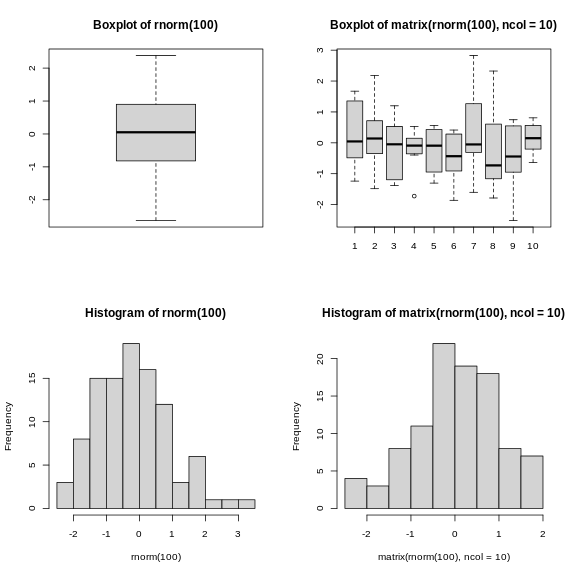
The out-of-the-box approach in base graphics can be very efficient
for simple, standard figures, that can be produced very quickly with a
single line of code and a single function such as plot, or
hist, or boxplot, … The defaults are however
not always the most appealing and tuning of figures, especially when
they become more complex (for example to produce facets), can become
lengthy and cumbersome.
The lattice package
The lattice package is similar to
ggplot2 in that is uses dataframes as input, returns
graphical objects and supports faceting. lattice however
isn’t based on the grammar of graphics and has a more convoluted
interface.
A good reference for the lattice package is @latticebook.
- Visualization in R
Source: Data Visualization Cheat Sheet.↩︎
Content from Next steps
Last updated on 2026-07-14 | Edit this page
Overview
Questions
- What is a
SummarizedExperiment? - What is Bioconductor?
Objectives
- Introduce the Bioconductor project.
- Introduce the notion of data containers.
- Give an overview of the
SummarizedExperiment, extensively used in omics analyses.
Next steps
Data in bioinformatics is often complex. To deal with this, developers define specialised data containers (termed classes) that match the properties of the data they need to handle.
This aspect is central to the Bioconductor1 project which uses the same core data infrastructure across packages. This certainly contributed to Bioconductor’s success. Bioconductor package developers are advised to make use of existing infrastructure to provide coherence, interoperability, and stability to the project as a whole.
To illustrate such an omics data container, we’ll present the
SummarizedExperiment class.
SummarizedExperiment
The figure below represents the anatomy of the SummarizedExperiment class.

Objects of the class SummarizedExperiment contain :
One (or more) assay(s) containing the quantitative omics data (expression data), stored as a matrix-like object. Features (genes, transcripts, proteins, …) are defined along the rows, and samples along the columns.
A sample metadata slot containing sample co-variates, stored as a data frame. Rows from this table represent samples (rows match exactly the columns of the expression data).
A feature metadata slot containing feature co-variates, stored as a data frame. The rows of this data frame match exactly the rows of the expression data.
The coordinated nature of the SummarizedExperiment
guarantees that during data manipulation, the dimensions of the
different slots will always match (i.e the columns in the expression
data and then rows in the sample metadata, as well as the rows in the
expression data and feature metadata) during data manipulation. For
example, if we had to exclude one sample from the assay, it would be
automatically removed from the sample metadata in the same
operation.
The metadata slots can grow additional co-variates (columns) without affecting the other structures.
Creating a SummarizedExperiment
In order to create a SummarizedExperiment, we will
create the individual components, i.e the count matrix, the sample and
gene metadata from csv files. These are typically how RNA-Seq data are
provided (after raw data have been processed).
-
An expression matrix: we load the count matrix,
specifying that the first columns contains row/gene names, and convert
the
data.frameto amatrix. You can download it by clicking this link.
R
count_matrix <- read.csv("data/count_matrix.csv",
row.names = 1) |>
as.matrix()
count_matrix[1:5, ]
OUTPUT
GSM2545336 GSM2545337 GSM2545338 GSM2545339 GSM2545340 GSM2545341
Asl 1170 361 400 586 626 988
Apod 36194 10347 9173 10620 13021 29594
Cyp2d22 4060 1616 1603 1901 2171 3349
Klk6 287 629 641 578 448 195
Fcrls 85 233 244 237 180 38
GSM2545342 GSM2545343 GSM2545344 GSM2545345 GSM2545346 GSM2545347
Asl 836 535 586 597 938 1035
Apod 24959 13668 13230 15868 27769 34301
Cyp2d22 3122 2008 2254 2277 2985 3452
Klk6 186 1101 537 567 327 233
Fcrls 68 375 199 177 89 67
GSM2545348 GSM2545349 GSM2545350 GSM2545351 GSM2545352 GSM2545353
Asl 494 481 666 937 803 541
Apod 11258 11812 15816 29242 20415 13682
Cyp2d22 1883 2014 2417 3678 2920 2216
Klk6 742 881 828 250 798 710
Fcrls 300 233 231 81 303 285
GSM2545354 GSM2545362 GSM2545363 GSM2545380
Asl 473 748 576 1192
Apod 11088 15916 11166 38148
Cyp2d22 1821 2842 2011 4019
Klk6 894 501 598 259
Fcrls 248 179 184 68R
dim(count_matrix)
OUTPUT
[1] 1474 22- A table describing the samples, available at this link.
R
sample_metadata <- read.csv("data/sample_metadata.csv")
sample_metadata
OUTPUT
sample organism age sex infection strain time tissue mouse
1 GSM2545336 Mus musculus 8 Female InfluenzaA C57BL/6 8 Cerebellum 14
2 GSM2545337 Mus musculus 8 Female NonInfected C57BL/6 0 Cerebellum 9
3 GSM2545338 Mus musculus 8 Female NonInfected C57BL/6 0 Cerebellum 10
4 GSM2545339 Mus musculus 8 Female InfluenzaA C57BL/6 4 Cerebellum 15
5 GSM2545340 Mus musculus 8 Male InfluenzaA C57BL/6 4 Cerebellum 18
6 GSM2545341 Mus musculus 8 Male InfluenzaA C57BL/6 8 Cerebellum 6
7 GSM2545342 Mus musculus 8 Female InfluenzaA C57BL/6 8 Cerebellum 5
8 GSM2545343 Mus musculus 8 Male NonInfected C57BL/6 0 Cerebellum 11
9 GSM2545344 Mus musculus 8 Female InfluenzaA C57BL/6 4 Cerebellum 22
10 GSM2545345 Mus musculus 8 Male InfluenzaA C57BL/6 4 Cerebellum 13
11 GSM2545346 Mus musculus 8 Male InfluenzaA C57BL/6 8 Cerebellum 23
12 GSM2545347 Mus musculus 8 Male InfluenzaA C57BL/6 8 Cerebellum 24
13 GSM2545348 Mus musculus 8 Female NonInfected C57BL/6 0 Cerebellum 8
14 GSM2545349 Mus musculus 8 Male NonInfected C57BL/6 0 Cerebellum 7
15 GSM2545350 Mus musculus 8 Male InfluenzaA C57BL/6 4 Cerebellum 1
16 GSM2545351 Mus musculus 8 Female InfluenzaA C57BL/6 8 Cerebellum 16
17 GSM2545352 Mus musculus 8 Female InfluenzaA C57BL/6 4 Cerebellum 21
18 GSM2545353 Mus musculus 8 Female NonInfected C57BL/6 0 Cerebellum 4
19 GSM2545354 Mus musculus 8 Male NonInfected C57BL/6 0 Cerebellum 2
20 GSM2545362 Mus musculus 8 Female InfluenzaA C57BL/6 4 Cerebellum 20
21 GSM2545363 Mus musculus 8 Male InfluenzaA C57BL/6 4 Cerebellum 12
22 GSM2545380 Mus musculus 8 Female InfluenzaA C57BL/6 8 Cerebellum 19R
dim(sample_metadata)
OUTPUT
[1] 22 9- A table describing the genes, available at this link.
R
gene_metadata <- read.csv("data/gene_metadata.csv")
gene_metadata[1:10, 1:4]
OUTPUT
gene ENTREZID
1 Asl 109900
2 Apod 11815
3 Cyp2d22 56448
4 Klk6 19144
5 Fcrls 80891
6 Slc2a4 20528
7 Exd2 97827
8 Gjc2 118454
9 Plp1 18823
10 Gnb4 14696
product
1 argininosuccinate lyase, transcript variant X1
2 apolipoprotein D, transcript variant 3
3 cytochrome P450, family 2, subfamily d, polypeptide 22, transcript variant 2
4 kallikrein related-peptidase 6, transcript variant 2
5 Fc receptor-like S, scavenger receptor, transcript variant X1
6 solute carrier family 2 (facilitated glucose transporter), member 4
7 exonuclease 3'-5' domain containing 2
8 gap junction protein, gamma 2, transcript variant 1
9 proteolipid protein (myelin) 1, transcript variant 1
10 guanine nucleotide binding protein (G protein), beta 4, transcript variant X2
ensembl_gene_id
1 ENSMUSG00000025533
2 ENSMUSG00000022548
3 ENSMUSG00000061740
4 ENSMUSG00000050063
5 ENSMUSG00000015852
6 ENSMUSG00000018566
7 ENSMUSG00000032705
8 ENSMUSG00000043448
9 ENSMUSG00000031425
10 ENSMUSG00000027669R
dim(gene_metadata)
OUTPUT
[1] 1474 9We will create a SummarizedExperiment from these
tables:
The count matrix that will be used as the
assayThe table describing the samples will be used as the sample metadata slot
The table describing the genes will be used as the features metadata slot
To do this we can put the different parts together using the
SummarizedExperiment constructor:
R
## BiocManager::install("SummarizedExperiment")
library("SummarizedExperiment")
First, we make sure that the samples are in the same order in the count matrix and the sample annotation, and the same for the genes in the count matrix and the gene annotation.
R
stopifnot(rownames(count_matrix) == gene_metadata$gene)
stopifnot(colnames(count_matrix) == sample_metadata$sample)
R
se <- SummarizedExperiment(assays = list(counts = count_matrix),
colData = sample_metadata,
rowData = gene_metadata)
se
OUTPUT
class: SummarizedExperiment
dim: 1474 22
metadata(0):
assays(1): counts
rownames(1474): Asl Apod ... Lmx1a Pbx1
rowData names(9): gene ENTREZID ... phenotype_description
hsapiens_homolog_associated_gene_name
colnames(22): GSM2545336 GSM2545337 ... GSM2545363 GSM2545380
colData names(9): sample organism ... tissue mouseSaving data
Exporting data to a spreadsheet, as we did in a previous episode, has
several limitations, such as those described in the first chapter
(possible inconsistencies with , and . for
decimal separators and lack of variable type definitions). Furthermore,
exporting data to a spreadsheet is only relevant for rectangular data
such as dataframes and matrices.
A more general way to save data, that is specific to R and is
guaranteed to work on any operating system, is to use the
saveRDS function. Saving objects like this will generate a
binary representation on disk (using the rds file extension
here), which can be loaded back into R using the readRDS
function.
R
saveRDS(se, file = "data_output/se.rds")
rm(se)
se <- readRDS("data_output/se.rds")
head(se)
To conclude, when it comes to saving data from R that will be loaded
again in R, saving and loading with saveRDS and
readRDS is the preferred approach. If tabular data need to
be shared with somebody that is not using R, then exporting to a
text-based spreadsheet is a good alternative.
Using this data structure, we can access the expression matrix with
the assay function:
R
head(assay(se))
OUTPUT
GSM2545336 GSM2545337 GSM2545338 GSM2545339 GSM2545340 GSM2545341
Asl 1170 361 400 586 626 988
Apod 36194 10347 9173 10620 13021 29594
Cyp2d22 4060 1616 1603 1901 2171 3349
Klk6 287 629 641 578 448 195
Fcrls 85 233 244 237 180 38
Slc2a4 782 231 248 265 313 786
GSM2545342 GSM2545343 GSM2545344 GSM2545345 GSM2545346 GSM2545347
Asl 836 535 586 597 938 1035
Apod 24959 13668 13230 15868 27769 34301
Cyp2d22 3122 2008 2254 2277 2985 3452
Klk6 186 1101 537 567 327 233
Fcrls 68 375 199 177 89 67
Slc2a4 528 249 266 357 654 693
GSM2545348 GSM2545349 GSM2545350 GSM2545351 GSM2545352 GSM2545353
Asl 494 481 666 937 803 541
Apod 11258 11812 15816 29242 20415 13682
Cyp2d22 1883 2014 2417 3678 2920 2216
Klk6 742 881 828 250 798 710
Fcrls 300 233 231 81 303 285
Slc2a4 271 304 349 715 513 320
GSM2545354 GSM2545362 GSM2545363 GSM2545380
Asl 473 748 576 1192
Apod 11088 15916 11166 38148
Cyp2d22 1821 2842 2011 4019
Klk6 894 501 598 259
Fcrls 248 179 184 68
Slc2a4 248 350 317 796R
dim(assay(se))
OUTPUT
[1] 1474 22We can access the sample metadata using the colData
function:
R
colData(se)
OUTPUT
DataFrame with 22 rows and 9 columns
sample organism age sex infection
<character> <character> <integer> <character> <character>
GSM2545336 GSM2545336 Mus musculus 8 Female InfluenzaA
GSM2545337 GSM2545337 Mus musculus 8 Female NonInfected
GSM2545338 GSM2545338 Mus musculus 8 Female NonInfected
GSM2545339 GSM2545339 Mus musculus 8 Female InfluenzaA
GSM2545340 GSM2545340 Mus musculus 8 Male InfluenzaA
... ... ... ... ... ...
GSM2545353 GSM2545353 Mus musculus 8 Female NonInfected
GSM2545354 GSM2545354 Mus musculus 8 Male NonInfected
GSM2545362 GSM2545362 Mus musculus 8 Female InfluenzaA
GSM2545363 GSM2545363 Mus musculus 8 Male InfluenzaA
GSM2545380 GSM2545380 Mus musculus 8 Female InfluenzaA
strain time tissue mouse
<character> <integer> <character> <integer>
GSM2545336 C57BL/6 8 Cerebellum 14
GSM2545337 C57BL/6 0 Cerebellum 9
GSM2545338 C57BL/6 0 Cerebellum 10
GSM2545339 C57BL/6 4 Cerebellum 15
GSM2545340 C57BL/6 4 Cerebellum 18
... ... ... ... ...
GSM2545353 C57BL/6 0 Cerebellum 4
GSM2545354 C57BL/6 0 Cerebellum 2
GSM2545362 C57BL/6 4 Cerebellum 20
GSM2545363 C57BL/6 4 Cerebellum 12
GSM2545380 C57BL/6 8 Cerebellum 19R
dim(colData(se))
OUTPUT
[1] 22 9We can also access the feature metadata using the
rowData function:
R
head(rowData(se))
OUTPUT
DataFrame with 6 rows and 9 columns
gene ENTREZID product ensembl_gene_id
<character> <integer> <character> <character>
Asl Asl 109900 argininosuccinate ly.. ENSMUSG00000025533
Apod Apod 11815 apolipoprotein D, tr.. ENSMUSG00000022548
Cyp2d22 Cyp2d22 56448 cytochrome P450, fam.. ENSMUSG00000061740
Klk6 Klk6 19144 kallikrein related-p.. ENSMUSG00000050063
Fcrls Fcrls 80891 Fc receptor-like S, .. ENSMUSG00000015852
Slc2a4 Slc2a4 20528 solute carrier famil.. ENSMUSG00000018566
external_synonym chromosome_name gene_biotype phenotype_description
<character> <character> <character> <character>
Asl 2510006M18Rik 5 protein_coding abnormal circulating..
Apod NA 16 protein_coding abnormal lipid homeo..
Cyp2d22 2D22 15 protein_coding abnormal skin morpho..
Klk6 Bssp 7 protein_coding abnormal cytokine le..
Fcrls 2810439C17Rik 3 protein_coding decreased CD8-positi..
Slc2a4 Glut-4 11 protein_coding abnormal circulating..
hsapiens_homolog_associated_gene_name
<character>
Asl ASL
Apod APOD
Cyp2d22 CYP2D6
Klk6 KLK6
Fcrls FCRL2
Slc2a4 SLC2A4R
dim(rowData(se))
OUTPUT
[1] 1474 9Subsetting a SummarizedExperiment
SummarizedExperiment can be subset just like with data frames, with numerics or with characters of logicals.
Below, we create a new instance of class SummarizedExperiment that contains only the 5 first features for the 3 first samples.
R
se1 <- se[1:5, 1:3]
se1
OUTPUT
class: SummarizedExperiment
dim: 5 3
metadata(0):
assays(1): counts
rownames(5): Asl Apod Cyp2d22 Klk6 Fcrls
rowData names(9): gene ENTREZID ... phenotype_description
hsapiens_homolog_associated_gene_name
colnames(3): GSM2545336 GSM2545337 GSM2545338
colData names(9): sample organism ... tissue mouseR
colData(se1)
OUTPUT
DataFrame with 3 rows and 9 columns
sample organism age sex infection
<character> <character> <integer> <character> <character>
GSM2545336 GSM2545336 Mus musculus 8 Female InfluenzaA
GSM2545337 GSM2545337 Mus musculus 8 Female NonInfected
GSM2545338 GSM2545338 Mus musculus 8 Female NonInfected
strain time tissue mouse
<character> <integer> <character> <integer>
GSM2545336 C57BL/6 8 Cerebellum 14
GSM2545337 C57BL/6 0 Cerebellum 9
GSM2545338 C57BL/6 0 Cerebellum 10R
rowData(se1)
OUTPUT
DataFrame with 5 rows and 9 columns
gene ENTREZID product ensembl_gene_id
<character> <integer> <character> <character>
Asl Asl 109900 argininosuccinate ly.. ENSMUSG00000025533
Apod Apod 11815 apolipoprotein D, tr.. ENSMUSG00000022548
Cyp2d22 Cyp2d22 56448 cytochrome P450, fam.. ENSMUSG00000061740
Klk6 Klk6 19144 kallikrein related-p.. ENSMUSG00000050063
Fcrls Fcrls 80891 Fc receptor-like S, .. ENSMUSG00000015852
external_synonym chromosome_name gene_biotype phenotype_description
<character> <character> <character> <character>
Asl 2510006M18Rik 5 protein_coding abnormal circulating..
Apod NA 16 protein_coding abnormal lipid homeo..
Cyp2d22 2D22 15 protein_coding abnormal skin morpho..
Klk6 Bssp 7 protein_coding abnormal cytokine le..
Fcrls 2810439C17Rik 3 protein_coding decreased CD8-positi..
hsapiens_homolog_associated_gene_name
<character>
Asl ASL
Apod APOD
Cyp2d22 CYP2D6
Klk6 KLK6
Fcrls FCRL2We can also use the colData() function to subset on
something from the sample metadata or the rowData() to
subset on something from the feature metadata. For example, here we keep
only miRNAs and the non infected samples:
R
se1 <- se[rowData(se)$gene_biotype == "miRNA",
colData(se)$infection == "NonInfected"]
se1
OUTPUT
class: SummarizedExperiment
dim: 7 7
metadata(0):
assays(1): counts
rownames(7): Mir1901 Mir378a ... Mir128-1 Mir7682
rowData names(9): gene ENTREZID ... phenotype_description
hsapiens_homolog_associated_gene_name
colnames(7): GSM2545337 GSM2545338 ... GSM2545353 GSM2545354
colData names(9): sample organism ... tissue mouseR
assay(se1)
OUTPUT
GSM2545337 GSM2545338 GSM2545343 GSM2545348 GSM2545349 GSM2545353
Mir1901 45 44 74 55 68 33
Mir378a 11 7 9 4 12 4
Mir133b 4 6 5 4 6 7
Mir30c-2 10 6 16 12 8 17
Mir149 1 2 0 0 0 0
Mir128-1 4 1 2 2 1 2
Mir7682 2 0 4 1 3 5
GSM2545354
Mir1901 60
Mir378a 8
Mir133b 3
Mir30c-2 15
Mir149 2
Mir128-1 1
Mir7682 5R
colData(se1)
OUTPUT
DataFrame with 7 rows and 9 columns
sample organism age sex infection
<character> <character> <integer> <character> <character>
GSM2545337 GSM2545337 Mus musculus 8 Female NonInfected
GSM2545338 GSM2545338 Mus musculus 8 Female NonInfected
GSM2545343 GSM2545343 Mus musculus 8 Male NonInfected
GSM2545348 GSM2545348 Mus musculus 8 Female NonInfected
GSM2545349 GSM2545349 Mus musculus 8 Male NonInfected
GSM2545353 GSM2545353 Mus musculus 8 Female NonInfected
GSM2545354 GSM2545354 Mus musculus 8 Male NonInfected
strain time tissue mouse
<character> <integer> <character> <integer>
GSM2545337 C57BL/6 0 Cerebellum 9
GSM2545338 C57BL/6 0 Cerebellum 10
GSM2545343 C57BL/6 0 Cerebellum 11
GSM2545348 C57BL/6 0 Cerebellum 8
GSM2545349 C57BL/6 0 Cerebellum 7
GSM2545353 C57BL/6 0 Cerebellum 4
GSM2545354 C57BL/6 0 Cerebellum 2R
rowData(se1)
OUTPUT
DataFrame with 7 rows and 9 columns
gene ENTREZID product ensembl_gene_id
<character> <integer> <character> <character>
Mir1901 Mir1901 100316686 microRNA 1901 ENSMUSG00000084565
Mir378a Mir378a 723889 microRNA 378a ENSMUSG00000105200
Mir133b Mir133b 723817 microRNA 133b ENSMUSG00000065480
Mir30c-2 Mir30c-2 723964 microRNA 30c-2 ENSMUSG00000065567
Mir149 Mir149 387167 microRNA 149 ENSMUSG00000065470
Mir128-1 Mir128-1 387147 microRNA 128-1 ENSMUSG00000065520
Mir7682 Mir7682 102466847 microRNA 7682 ENSMUSG00000106406
external_synonym chromosome_name gene_biotype phenotype_description
<character> <character> <character> <character>
Mir1901 Mirn1901 18 miRNA NA
Mir378a Mirn378 18 miRNA abnormal mitochondri..
Mir133b mir 133b 1 miRNA no abnormal phenotyp..
Mir30c-2 mir 30c-2 1 miRNA NA
Mir149 Mirn149 1 miRNA increased circulatin..
Mir128-1 Mirn128 1 miRNA no abnormal phenotyp..
Mir7682 mmu-mir-7682 1 miRNA NA
hsapiens_homolog_associated_gene_name
<character>
Mir1901 NA
Mir378a MIR378A
Mir133b MIR133B
Mir30c-2 MIR30C2
Mir149 NA
Mir128-1 MIR128-1
Mir7682 NAChallenge
Extract the gene expression levels of the 3 first genes in samples at time 0 and at time 8.
R
assay(se)[1:3, colData(se)$time != 4]
OUTPUT
GSM2545336 GSM2545337 GSM2545338 GSM2545341 GSM2545342 GSM2545343
Asl 1170 361 400 988 836 535
Apod 36194 10347 9173 29594 24959 13668
Cyp2d22 4060 1616 1603 3349 3122 2008
GSM2545346 GSM2545347 GSM2545348 GSM2545349 GSM2545351 GSM2545353
Asl 938 1035 494 481 937 541
Apod 27769 34301 11258 11812 29242 13682
Cyp2d22 2985 3452 1883 2014 3678 2216
GSM2545354 GSM2545380
Asl 473 1192
Apod 11088 38148
Cyp2d22 1821 4019R
# Equivalent to
assay(se)[1:3, colData(se)$time == 0 | colData(se)$time == 8]
OUTPUT
GSM2545336 GSM2545337 GSM2545338 GSM2545341 GSM2545342 GSM2545343
Asl 1170 361 400 988 836 535
Apod 36194 10347 9173 29594 24959 13668
Cyp2d22 4060 1616 1603 3349 3122 2008
GSM2545346 GSM2545347 GSM2545348 GSM2545349 GSM2545351 GSM2545353
Asl 938 1035 494 481 937 541
Apod 27769 34301 11258 11812 29242 13682
Cyp2d22 2985 3452 1883 2014 3678 2216
GSM2545354 GSM2545380
Asl 473 1192
Apod 11088 38148
Cyp2d22 1821 4019Challenge
Verify that you get the same values using the long rna
table.
R
rna |>
filter(gene %in% c("Asl", "Apod", "Cyd2d22")) |>
filter(time != 4) |>
select(expression)
OUTPUT
# A tibble: 28 × 1
expression
<dbl>
1 1170
2 36194
3 361
4 10347
5 400
6 9173
7 988
8 29594
9 836
10 24959
# ℹ 18 more rowsThe long table and the SummarizedExperiment contain the
same information, but are simply structured differently. Each approach
has its own advantages: the former is a good fit for the
tidyverse packages, while the latter is the preferred
structure for many bioinformatics and statistical processing steps. For
example, a typical RNA-Seq analyses using the DESeq2
package.
Adding variables to metadata
We can also add information to the metadata. Suppose that you want to add the center where the samples were collected…
R
colData(se)$center <- rep("University of Illinois", nrow(colData(se)))
colData(se)
OUTPUT
DataFrame with 22 rows and 10 columns
sample organism age sex infection
<character> <character> <integer> <character> <character>
GSM2545336 GSM2545336 Mus musculus 8 Female InfluenzaA
GSM2545337 GSM2545337 Mus musculus 8 Female NonInfected
GSM2545338 GSM2545338 Mus musculus 8 Female NonInfected
GSM2545339 GSM2545339 Mus musculus 8 Female InfluenzaA
GSM2545340 GSM2545340 Mus musculus 8 Male InfluenzaA
... ... ... ... ... ...
GSM2545353 GSM2545353 Mus musculus 8 Female NonInfected
GSM2545354 GSM2545354 Mus musculus 8 Male NonInfected
GSM2545362 GSM2545362 Mus musculus 8 Female InfluenzaA
GSM2545363 GSM2545363 Mus musculus 8 Male InfluenzaA
GSM2545380 GSM2545380 Mus musculus 8 Female InfluenzaA
strain time tissue mouse center
<character> <integer> <character> <integer> <character>
GSM2545336 C57BL/6 8 Cerebellum 14 University of Illinois
GSM2545337 C57BL/6 0 Cerebellum 9 University of Illinois
GSM2545338 C57BL/6 0 Cerebellum 10 University of Illinois
GSM2545339 C57BL/6 4 Cerebellum 15 University of Illinois
GSM2545340 C57BL/6 4 Cerebellum 18 University of Illinois
... ... ... ... ... ...
GSM2545353 C57BL/6 0 Cerebellum 4 University of Illinois
GSM2545354 C57BL/6 0 Cerebellum 2 University of Illinois
GSM2545362 C57BL/6 4 Cerebellum 20 University of Illinois
GSM2545363 C57BL/6 4 Cerebellum 12 University of Illinois
GSM2545380 C57BL/6 8 Cerebellum 19 University of IllinoisThis illustrates that the metadata slots can grow indefinitely without affecting the other structures!
tidySummarizedExperiment
You may be wondering, can we use tidyverse commands to interact with
SummarizedExperiment objects? The answer is yes, we can
with the tidySummarizedExperiment package.
Remember what our SummarizedExperiment object looks like:
R
se
OUTPUT
class: SummarizedExperiment
dim: 1474 22
metadata(0):
assays(1): counts
rownames(1474): Asl Apod ... Lmx1a Pbx1
rowData names(9): gene ENTREZID ... phenotype_description
hsapiens_homolog_associated_gene_name
colnames(22): GSM2545336 GSM2545337 ... GSM2545363 GSM2545380
colData names(10): sample organism ... mouse centerLoad tidySummarizedExperiment and then take a look at
the se object again.
R
#BiocManager::install("tidySummarizedExperiment")
library("tidySummarizedExperiment")
se
OUTPUT
class: SummarizedExperiment
dim: 1474 22
metadata(0):
assays(1): counts
rownames(1474): Asl Apod ... Lmx1a Pbx1
rowData names(9): gene ENTREZID ... phenotype_description
hsapiens_homolog_associated_gene_name
colnames(22): GSM2545336 GSM2545337 ... GSM2545363 GSM2545380
colData names(10): sample organism ... mouse centerIt’s still a SummarizedExperiment object, so maintains
the efficient structure, but now we can view it as a tibble. Note the
first line of the output says this, it’s a
SummarizedExperiment-tibble abstraction. We
can also see in the second line of the output the number of transcripts
and samples.
If we want to revert to the standard
SummarizedExperiment view, we can do that.
R
options("restore_SummarizedExperiment_show" = TRUE)
se
OUTPUT
class: SummarizedExperiment
dim: 1474 22
metadata(0):
assays(1): counts
rownames(1474): Asl Apod ... Lmx1a Pbx1
rowData names(9): gene ENTREZID ... phenotype_description
hsapiens_homolog_associated_gene_name
colnames(22): GSM2545336 GSM2545337 ... GSM2545363 GSM2545380
colData names(10): sample organism ... mouse centerBut here we use the tibble view.
R
options("restore_SummarizedExperiment_show" = FALSE)
se
OUTPUT
class: SummarizedExperiment
dim: 1474 22
metadata(0):
assays(1): counts
rownames(1474): Asl Apod ... Lmx1a Pbx1
rowData names(9): gene ENTREZID ... phenotype_description
hsapiens_homolog_associated_gene_name
colnames(22): GSM2545336 GSM2545337 ... GSM2545363 GSM2545380
colData names(10): sample organism ... mouse centerWe can now use tidyverse commands to interact with the
SummarizedExperiment object.
We can use filter to filter for rows using a condition
e.g. to view all rows for one sample.
R
se |> filter(.sample == "GSM2545336")
ERROR
Error in `dplyr_fn()` at tidySummarizedExperiment/R/query_scope_analysis.R:481:3:
ℹ In argument: `.sample == "GSM2545336"`.
Caused by error:
! object '.sample' not foundWe can use select to specify columns we want to
view.
R
se |> select(.sample)
WARNING
Warning: `when()` was deprecated in purrr 1.0.0.
ℹ Please use `if` instead.
ℹ The deprecated feature was likely used in the tidySummarizedExperiment
package.
Please report the issue at
<https://github.com/stemangiola/tidySummarizedExperiment/issues>.
This warning is displayed once per session.
Call `lifecycle::last_lifecycle_warnings()` to see where this warning was
generated.OUTPUT
tidySummarizedExperiment says: Key columns are missing. A data frame is returned for independent data analysis.OUTPUT
# A tibble: 32,428 × 1
.sample
<chr>
1 GSM2545336
2 GSM2545336
3 GSM2545336
4 GSM2545336
5 GSM2545336
6 GSM2545336
7 GSM2545336
8 GSM2545336
9 GSM2545336
10 GSM2545336
# ℹ 32,418 more rowsWe can use mutate to add metadata info.
R
se |> mutate(center = "Heidelberg University")
OUTPUT
class: SummarizedExperiment
dim: 1474 22
metadata(1): latest_mutate_scope_report
assays(1): counts
rownames(1474): Asl Apod ... Lmx1a Pbx1
rowData names(9): gene ENTREZID ... phenotype_description
hsapiens_homolog_associated_gene_name
colnames(22): GSM2545336 GSM2545337 ... GSM2545363 GSM2545380
colData names(10): sample organism ... mouse centerWe can also combine commands with the tidyverse pipe
|>. For example, we could combine group_by
and summarise to get the total counts for each sample.
R
se |>
group_by(.sample) |>
summarise(total_counts=sum(counts))
OUTPUT
tidySummarizedExperiment says: A data frame is returned for independent data analysis.OUTPUT
# A tibble: 22 × 2
.sample total_counts
<chr> <int>
1 GSM2545336 3039671
2 GSM2545337 2602360
3 GSM2545338 2458618
4 GSM2545339 2500082
5 GSM2545340 2479024
6 GSM2545341 2413723
7 GSM2545342 2349728
8 GSM2545343 3105652
9 GSM2545344 2524137
10 GSM2545345 2506038
# ℹ 12 more rowsWe can treat the tidy SummarizedExperiment object as a normal tibble for plotting.
Here we plot the distribution of counts per sample.
R
se |>
ggplot(aes(counts + 1, group=.sample, color=infection)) +
geom_density() +
scale_x_log10() +
theme_bw()
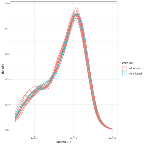
For more information on tidySummarizedExperiment, see
the package
website.
Take-home message
SummarizedExperimentrepresents an efficient way to store and handle omics data.They are used in many Bioconductor packages.
If you follow the next training focused on RNA sequencing analysis,
you will learn to use the Bioconductor DESeq2 package to do
some differential expression analyses. The whole analysis of the
DESeq2 package is handled in a
SummarizedExperiment.
- Bioconductor is a project provide support and packages for the comprehension of high high-throughput biology data.
- A
SummarizedExperimentis a type of object useful to store and manage high-throughput omics data.
The Bioconductor was initiated by Robert Gentleman, one of the two creators of the R language. Bioconductor provides tools dedicated to omics data analysis. Bioconductor uses the R statistical programming language and is open source and open development.↩︎