Manipulating and analysing data with dplyr
Last updated on 2026-04-21 | Edit this page
Overview
Questions
- Data analysis in R using the tidyverse meta-package
Objectives
- Describe the purpose of the
dplyrandtidyrpackages. - Describe several of their functions that are extremely useful to manipulate data.
- Describe the concept of a wide and a long table format, and see how to reshape a data frame from one format to the other one.
- Demonstrate how to join tables.
This episode is based on the Data Carpentries’s Data Analysis and Visualisation in R for Ecologists lesson.
Data manipulation using dplyr and
tidyr
Bracket subsetting is handy, but it can be cumbersome and difficult to read, especially for complicated operations.
Some packages can greatly facilitate our task when we manipulate
data. Packages in R are basically sets of additional functions that let
you do more stuff. The functions we’ve been using so far, like
str() or data.frame(), come built into R;
Loading packages can give you access to other specific functions. Before
you use a package for the first time you need to install it on your
machine, and then you should import it in every subsequent R session
when you need it.
The package
dplyrprovides powerful tools for data manipulation tasks. It is built to work directly with data frames, with many manipulation tasks optimised.As we will see latter on, sometimes we want a data frame to be reshaped to be able to do some specific analyses or for visualisation. The package
tidyraddresses this common problem of reshaping data and provides tools for manipulating data in a tidy way.
To learn more about dplyr and
tidyr after the workshop, you may want to
check out this handy
data transformation with dplyr
cheatsheet and this one
about tidyr.
- The
tidyversepackage is an “umbrella-package” that installs several useful packages for data analysis which work well together, such astidyr,dplyr,ggplot2,tibble, etc. These packages help us to work and interact with the data. They allow us to do many things with your data, such as subsetting, transforming, visualising, etc.
If you did the set up, you should have already installed the tidyverse package. Check to see if you have it by trying to load in from the library:
R
## load the tidyverse packages, incl. dplyr
library("tidyverse")
If you got an error message
there is no package called ‘tidyverse’ then you have not
installed the package yet for this version of R. To install the
tidyverse package type:
R
BiocManager::install("tidyverse")
If you had to install the tidyverse
package, do not forget to load it in this R session by using the
library() command above!
Loading data with tidyverse
Instead of read.csv(), we will read in our data using
the read_csv() function (notice the _ instead
of the .), from the tidyverse package
readr.
R
rna <- read_csv("data/rnaseq.csv")

## view the data
rna
OUTPUT
# A tibble: 32,428 × 19
   gene    sample  expression organism   age sex   infection strain  time tissue
   <chr>   <chr>        <dbl> <chr>    <dbl> <chr> <chr>     <chr>  <dbl> <chr>
 1 Asl     GSM254…       1170 Mus mus…     8 Fema… Influenz… C57BL…     8 Cereb…
 2 Apod    GSM254…      36194 Mus mus…     8 Fema… Influenz… C57BL…     8 Cereb…
 3 Cyp2d22 GSM254…       4060 Mus mus…     8 Fema… Influenz… C57BL…     8 Cereb…
 4 Klk6    GSM254…        287 Mus mus…     8 Fema… Influenz… C57BL…     8 Cereb…
 5 Fcrls   GSM254…         85 Mus mus…     8 Fema… Influenz… C57BL…     8 Cereb…
 6 Slc2a4  GSM254…        782 Mus mus…     8 Fema… Influenz… C57BL…     8 Cereb…
 7 Exd2    GSM254…       1619 Mus mus…     8 Fema… Influenz… C57BL…     8 Cereb…
 8 Gjc2    GSM254…        288 Mus mus…     8 Fema… Influenz… C57BL…     8 Cereb…
 9 Plp1    GSM254…      43217 Mus mus…     8 Fema… Influenz… C57BL…     8 Cereb…
10 Gnb4    GSM254…       1071 Mus mus…     8 Fema… Influenz… C57BL…     8 Cereb…
# ℹ 32,418 more rows
# ℹ 9 more variables: mouse <dbl>, ENTREZID <dbl>, product <chr>,
#   ensembl_gene_id <chr>, external_synonym <chr>, chromosome_name <chr>,
#   gene_biotype <chr>, phenotype_description <chr>,
#   hsapiens_homolog_associated_gene_name <chr>
Notice that the class of the data is now referred to as a “tibble”.
Tibbles tweak some of the behaviors of the data frame objects we introduced in the previously. The data structure is very similar to a data frame. For our purposes the only differences are that:
It displays the data type of each column under its name. Note that <
dbl> is a data type defined to hold numeric values with decimal points.It only prints the first few rows of data and only as many columns as fit on one screen.
We are now going to learn some of the most common
dplyr functions:
-
select(): subset columns -
filter(): subset rows on conditions -
mutate(): create new columns by using information from other columns -
group_by()andsummarise(): create summary statistics on grouped data -
arrange(): sort results -
count(): count discrete values
Selecting columns and filtering rows
To select columns of a data frame, use select(). The
first argument to this function is the data frame (rna),
and the subsequent arguments are the columns to keep.
R
select(rna, gene, sample, tissue, expression)
OUTPUT
# A tibble: 32,428 × 4
   gene    sample     tissue     expression
   <chr>   <chr>      <chr>           <dbl>
 1 Asl     GSM2545336 Cerebellum       1170
 2 Apod    GSM2545336 Cerebellum      36194
 3 Cyp2d22 GSM2545336 Cerebellum       4060
 4 Klk6    GSM2545336 Cerebellum        287
 5 Fcrls   GSM2545336 Cerebellum         85
 6 Slc2a4  GSM2545336 Cerebellum        782
 7 Exd2    GSM2545336 Cerebellum       1619
 8 Gjc2    GSM2545336 Cerebellum        288
 9 Plp1    GSM2545336 Cerebellum      43217
10 Gnb4    GSM2545336 Cerebellum       1071
# ℹ 32,418 more rows
To select all columns except certain ones, put a “-” in front of the variable to exclude it.
R
select(rna, -tissue, -organism)
OUTPUT
# A tibble: 32,428 × 17
   gene    sample   expression   age sex   infection strain  time mouse ENTREZID
   <chr>   <chr>         <dbl> <dbl> <chr> <chr>     <chr>  <dbl> <dbl>    <dbl>
 1 Asl     GSM2545…       1170     8 Fema… Influenz… C57BL…     8    14   109900
 2 Apod    GSM2545…      36194     8 Fema… Influenz… C57BL…     8    14    11815
 3 Cyp2d22 GSM2545…       4060     8 Fema… Influenz… C57BL…     8    14    56448
 4 Klk6    GSM2545…        287     8 Fema… Influenz… C57BL…     8    14    19144
 5 Fcrls   GSM2545…         85     8 Fema… Influenz… C57BL…     8    14    80891
 6 Slc2a4  GSM2545…        782     8 Fema… Influenz… C57BL…     8    14    20528
 7 Exd2    GSM2545…       1619     8 Fema… Influenz… C57BL…     8    14    97827
 8 Gjc2    GSM2545…        288     8 Fema… Influenz… C57BL…     8    14   118454
 9 Plp1    GSM2545…      43217     8 Fema… Influenz… C57BL…     8    14    18823
10 Gnb4    GSM2545…       1071     8 Fema… Influenz… C57BL…     8    14    14696
# ℹ 32,418 more rows
# ℹ 7 more variables: product <chr>, ensembl_gene_id <chr>,
#   external_synonym <chr>, chromosome_name <chr>, gene_biotype <chr>,
#   phenotype_description <chr>, hsapiens_homolog_associated_gene_name <chr>
This will select all the variables in rna except
tissue and organism.
To choose rows based on a specific criteria, use
filter():
R
filter(rna, sex == "Male")
OUTPUT
# A tibble: 14,740 × 19
   gene    sample  expression organism   age sex   infection strain  time tissue
   <chr>   <chr>        <dbl> <chr>    <dbl> <chr> <chr>     <chr>  <dbl> <chr>
 1 Asl     GSM254…        626 Mus mus…     8 Male  Influenz… C57BL…     4 Cereb…
 2 Apod    GSM254…      13021 Mus mus…     8 Male  Influenz… C57BL…     4 Cereb…
 3 Cyp2d22 GSM254…       2171 Mus mus…     8 Male  Influenz… C57BL…     4 Cereb…
 4 Klk6    GSM254…        448 Mus mus…     8 Male  Influenz… C57BL…     4 Cereb…
 5 Fcrls   GSM254…        180 Mus mus…     8 Male  Influenz… C57BL…     4 Cereb…
 6 Slc2a4  GSM254…        313 Mus mus…     8 Male  Influenz… C57BL…     4 Cereb…
 7 Exd2    GSM254…       2366 Mus mus…     8 Male  Influenz… C57BL…     4 Cereb…
 8 Gjc2    GSM254…        310 Mus mus…     8 Male  Influenz… C57BL…     4 Cereb…
 9 Plp1    GSM254…      53126 Mus mus…     8 Male  Influenz… C57BL…     4 Cereb…
10 Gnb4    GSM254…       1355 Mus mus…     8 Male  Influenz… C57BL…     4 Cereb…
# ℹ 14,730 more rows
# ℹ 9 more variables: mouse <dbl>, ENTREZID <dbl>, product <chr>,
#   ensembl_gene_id <chr>, external_synonym <chr>, chromosome_name <chr>,
#   gene_biotype <chr>, phenotype_description <chr>,
#   hsapiens_homolog_associated_gene_name <chr>
R
filter(rna, sex == "Male" & infection == "NonInfected")
OUTPUT
# A tibble: 4,422 × 19
   gene    sample  expression organism   age sex   infection strain  time tissue
   <chr>   <chr>        <dbl> <chr>    <dbl> <chr> <chr>     <chr>  <dbl> <chr>
 1 Asl     GSM254…        535 Mus mus…     8 Male  NonInfec… C57BL…     0 Cereb…
 2 Apod    GSM254…      13668 Mus mus…     8 Male  NonInfec… C57BL…     0 Cereb…
 3 Cyp2d22 GSM254…       2008 Mus mus…     8 Male  NonInfec… C57BL…     0 Cereb…
 4 Klk6    GSM254…       1101 Mus mus…     8 Male  NonInfec… C57BL…     0 Cereb…
 5 Fcrls   GSM254…        375 Mus mus…     8 Male  NonInfec… C57BL…     0 Cereb…
 6 Slc2a4  GSM254…        249 Mus mus…     8 Male  NonInfec… C57BL…     0 Cereb…
 7 Exd2    GSM254…       3126 Mus mus…     8 Male  NonInfec… C57BL…     0 Cereb…
 8 Gjc2    GSM254…        791 Mus mus…     8 Male  NonInfec… C57BL…     0 Cereb…
 9 Plp1    GSM254…      98658 Mus mus…     8 Male  NonInfec… C57BL…     0 Cereb…
10 Gnb4    GSM254…       2437 Mus mus…     8 Male  NonInfec… C57BL…     0 Cereb…
# ℹ 4,412 more rows
# ℹ 9 more variables: mouse <dbl>, ENTREZID <dbl>, product <chr>,
#   ensembl_gene_id <chr>, external_synonym <chr>, chromosome_name <chr>,
#   gene_biotype <chr>, phenotype_description <chr>,
#   hsapiens_homolog_associated_gene_name <chr>
Now let’s imagine we are interested in the human homologs of the
mouse genes analysed in this dataset. This information can be found in
the last column of the rna tibble, named
hsapiens_homolog_associated_gene_name. To visualise it
easily, we will create a new table containing just the 2 columns
gene and
hsapiens_homolog_associated_gene_name.
R
genes <- select(rna, gene, hsapiens_homolog_associated_gene_name)
genes
OUTPUT
# A tibble: 32,428 × 2
   gene    hsapiens_homolog_associated_gene_name
   <chr>   <chr>
 1 Asl     ASL
 2 Apod    APOD
 3 Cyp2d22 CYP2D6
 4 Klk6    KLK6
 5 Fcrls   FCRL2
 6 Slc2a4  SLC2A4
 7 Exd2    EXD2
 8 Gjc2    GJC2
 9 Plp1    PLP1
10 Gnb4    GNB4
# ℹ 32,418 more rows
Some mouse genes have no human homologs. These can be retrieved using
filter() and the is.na() function, that
determines whether something is an NA.
R
filter(genes, is.na(hsapiens_homolog_associated_gene_name))
OUTPUT
# A tibble: 4,290 × 2
   gene     hsapiens_homolog_associated_gene_name
   <chr>    <chr>
 1 Prodh    <NA>
 2 Tssk5    <NA>
 3 Vmn2r1   <NA>
 4 Gm10654  <NA>
 5 Hexa     <NA>
 6 Sult1a1  <NA>
 7 Gm6277   <NA>
 8 Tmem198b <NA>
 9 Adam1a   <NA>
10 Ebp      <NA>
# ℹ 4,280 more rows
If we want to keep only mouse genes that have a human homolog, we can
insert a “!” symbol that negates the result, so we’re asking for every
row where hsapiens_homolog_associated_gene_name is not an
NA.
R
filter(genes, !is.na(hsapiens_homolog_associated_gene_name))
OUTPUT
# A tibble: 28,138 × 2
   gene    hsapiens_homolog_associated_gene_name
   <chr>   <chr>
 1 Asl     ASL
 2 Apod    APOD
 3 Cyp2d22 CYP2D6
 4 Klk6    KLK6
 5 Fcrls   FCRL2
 6 Slc2a4  SLC2A4
 7 Exd2    EXD2
 8 Gjc2    GJC2
 9 Plp1    PLP1
10 Gnb4    GNB4
# ℹ 28,128 more rows
Pipes
What if you want to select and filter at the same time? There are three ways to do this: use intermediate steps, nested functions, or pipes.
With intermediate steps, you create a temporary data frame and use that as input to the next function, like this:
R
rna2 <- filter(rna, sex == "Male")
rna3 <- select(rna2, gene, sample, tissue, expression)
rna3
OUTPUT
# A tibble: 14,740 × 4
   gene    sample     tissue     expression
   <chr>   <chr>      <chr>           <dbl>
 1 Asl     GSM2545340 Cerebellum        626
 2 Apod    GSM2545340 Cerebellum      13021
 3 Cyp2d22 GSM2545340 Cerebellum       2171
 4 Klk6    GSM2545340 Cerebellum        448
 5 Fcrls   GSM2545340 Cerebellum        180
 6 Slc2a4  GSM2545340 Cerebellum        313
 7 Exd2    GSM2545340 Cerebellum       2366
 8 Gjc2    GSM2545340 Cerebellum        310
 9 Plp1    GSM2545340 Cerebellum      53126
10 Gnb4    GSM2545340 Cerebellum       1355
# ℹ 14,730 more rows
This is readable, but can clutter up your workspace with lots of intermediate objects that you have to name individually. With multiple steps, that can be hard to keep track of.
You can also nest functions (i.e. one function inside of another), like this:
R
rna3 <- select(filter(rna, sex == "Male"), gene, sample, tissue, expression)
rna3
OUTPUT
# A tibble: 14,740 × 4
   gene    sample     tissue     expression
   <chr>   <chr>      <chr>           <dbl>
 1 Asl     GSM2545340 Cerebellum        626
 2 Apod    GSM2545340 Cerebellum      13021
 3 Cyp2d22 GSM2545340 Cerebellum       2171
 4 Klk6    GSM2545340 Cerebellum        448
 5 Fcrls   GSM2545340 Cerebellum        180
 6 Slc2a4  GSM2545340 Cerebellum        313
 7 Exd2    GSM2545340 Cerebellum       2366
 8 Gjc2    GSM2545340 Cerebellum        310
 9 Plp1    GSM2545340 Cerebellum      53126
10 Gnb4    GSM2545340 Cerebellum       1355
# ℹ 14,730 more rows
This is handy, but can be difficult to read if too many functions are nested, as R evaluates the expression from the inside out (in this case, filtering, then selecting).
The last option, pipes, are a recent addition to R. Pipes let you take the output of one function and send it directly to the next, which is useful when you need to do many things to the same dataset.
Pipes in R look like %>% (made available via the
magrittr package) or |>
(through base R). If you use RStudio, you can type the pipe with
Ctrl + Shift + M if you have a PC or
Cmd + Shift + M if you have a Mac.
In the above code, we use the pipe to send the rna
dataset first through filter() to keep rows where
sex is Male, then through select() to keep
only the gene, sample, tissue,
and expressioncolumns.
The pipe |> takes the object on its left and passes
it directly as the first argument to the function on its right, we don’t
need to explicitly include the data frame as an argument to the
filter() and select() functions any more.
R
rna |>
  filter(sex == "Male") |>
  select(gene, sample, tissue, expression)
OUTPUT
# A tibble: 14,740 × 4
   gene    sample     tissue     expression
   <chr>   <chr>      <chr>           <dbl>
 1 Asl     GSM2545340 Cerebellum        626
 2 Apod    GSM2545340 Cerebellum      13021
 3 Cyp2d22 GSM2545340 Cerebellum       2171
 4 Klk6    GSM2545340 Cerebellum        448
 5 Fcrls   GSM2545340 Cerebellum        180
 6 Slc2a4  GSM2545340 Cerebellum        313
 7 Exd2    GSM2545340 Cerebellum       2366
 8 Gjc2    GSM2545340 Cerebellum        310
 9 Plp1    GSM2545340 Cerebellum      53126
10 Gnb4    GSM2545340 Cerebellum       1355
# ℹ 14,730 more rows
Some may find it helpful to read the pipe like the word “then”. For
instance, in the above example, we took the data frame rna,
then we filtered for rows with
sex == "Male", then we selected
columns gene, sample, tissue, and
expression.
The dplyr functions by themselves are
somewhat simple, but by combining them into linear workflows with the
pipe, we can accomplish more complex manipulations of data frames.
If we want to create a new object with this smaller version of the data, we can assign it a new name:
R
rna3 <- rna |>
  filter(sex == "Male") |>
  select(gene, sample, tissue, expression)

rna3
OUTPUT
# A tibble: 14,740 × 4
   gene    sample     tissue     expression
   <chr>   <chr>      <chr>           <dbl>
 1 Asl     GSM2545340 Cerebellum        626
 2 Apod    GSM2545340 Cerebellum      13021
 3 Cyp2d22 GSM2545340 Cerebellum       2171
 4 Klk6    GSM2545340 Cerebellum        448
 5 Fcrls   GSM2545340 Cerebellum        180
 6 Slc2a4  GSM2545340 Cerebellum        313
 7 Exd2    GSM2545340 Cerebellum       2366
 8 Gjc2    GSM2545340 Cerebellum        310
 9 Plp1    GSM2545340 Cerebellum      53126
10 Gnb4    GSM2545340 Cerebellum       1355
# ℹ 14,730 more rowsChallenge:
Using pipes, subset the rna data to keep observations in
female mice at time 0, where the gene has an expression higher than
50000, and retain only the columns gene,
sample, time, expression and
age.
R
rna |>
  filter(expression > 50000,
         sex == "Female",
         time == 0 ) |>
  select(gene, sample, time, expression, age)
OUTPUT
# A tibble: 9 × 5
  gene   sample      time expression   age
  <chr>  <chr>      <dbl>      <dbl> <dbl>
1 Plp1   GSM2545337     0     101241     8
2 Atp1b1 GSM2545337     0      53260     8
3 Plp1   GSM2545338     0      96534     8
4 Atp1b1 GSM2545338     0      50614     8
5 Plp1   GSM2545348     0     102790     8
6 Atp1b1 GSM2545348     0      59544     8
7 Plp1   GSM2545353     0      71237     8
8 Glul   GSM2545353     0      52451     8
9 Atp1b1 GSM2545353     0      61451     8
Mutate
Frequently you’ll want to create new columns based on the values of
existing columns, for example to do unit conversions, or to find the
ratio of values in two columns. For this we’ll use
mutate().
To create a new column of time in hours:
R
rna |>
  mutate(time_hours = time * 24) |>
  select(time, time_hours)
OUTPUT
# A tibble: 32,428 × 2
    time time_hours
   <dbl>      <dbl>
 1     8        192
 2     8        192
 3     8        192
 4     8        192
 5     8        192
 6     8        192
 7     8        192
 8     8        192
 9     8        192
10     8        192
# ℹ 32,418 more rows
You can also create a second new column based on the first new column
within the same call of mutate():
R
rna |>
  mutate(time_hours = time * 24,
         time_mn = time_hours * 60) |>
  select(time, time_hours, time_mn)
OUTPUT
# A tibble: 32,428 × 3
    time time_hours time_mn
   <dbl>      <dbl>   <dbl>
 1     8        192   11520
 2     8        192   11520
 3     8        192   11520
 4     8        192   11520
 5     8        192   11520
 6     8        192   11520
 7     8        192   11520
 8     8        192   11520
 9     8        192   11520
10     8        192   11520
# ℹ 32,418 more rows
Challenge
Create a new data frame from the rna data that meets the
following criteria: contains only the gene,
chromosome_name, phenotype_description,
sample, and expression columns. The expression
values should be log-transformed. This data frame must only contain
genes located on sex chromosomes, associated with a
phenotype_description, and with a log expression higher than 5.
Hint: think about how the commands should be ordered to produce this data frame!
R
rna |>
  mutate(expression = log(expression)) |>
  select(gene, chromosome_name, phenotype_description, sample, expression) |>
  filter(chromosome_name == "X" | chromosome_name == "Y") |>
  filter(!is.na(phenotype_description)) |>
  filter(expression > 5)
OUTPUT
# A tibble: 649 × 5
   gene   chromosome_name phenotype_description                sample expression
   <chr>  <chr>           <chr>                                <chr>       <dbl>
 1 Plp1   X               abnormal CNS glial cell morphology   GSM25…      10.7
 2 Slc7a3 X               decreased body length                GSM25…       5.46
 3 Plxnb3 X               abnormal coat appearance             GSM25…       6.58
 4 Rbm3   X               abnormal liver morphology            GSM25…       9.32
 5 Cfp    X               abnormal cardiovascular system phys… GSM25…       6.18
 6 Ebp    X               abnormal embryonic erythrocyte morp… GSM25…       6.68
 7 Cd99l2 X               abnormal cellular extravasation      GSM25…       8.04
 8 Piga   X               abnormal brain development           GSM25…       6.06
 9 Pim2   X               decreased T cell proliferation       GSM25…       7.11
10 Itm2a  X               no abnormal phenotype detected       GSM25…       7.48
# ℹ 639 more rows
Split-apply-combine data analysis
Many data analysis tasks can be approached using the
split-apply-combine paradigm: split the data into groups, apply
some analysis to each group, and then combine the results.
dplyr makes this very easy through the use
of the group_by() function.
R
rna |>
  group_by(gene)
OUTPUT
# A tibble: 32,428 × 19
# Groups:   gene [1,474]
   gene    sample  expression organism   age sex   infection strain  time tissue
   <chr>   <chr>        <dbl> <chr>    <dbl> <chr> <chr>     <chr>  <dbl> <chr>
 1 Asl     GSM254…       1170 Mus mus…     8 Fema… Influenz… C57BL…     8 Cereb…
 2 Apod    GSM254…      36194 Mus mus…     8 Fema… Influenz… C57BL…     8 Cereb…
 3 Cyp2d22 GSM254…       4060 Mus mus…     8 Fema… Influenz… C57BL…     8 Cereb…
 4 Klk6    GSM254…        287 Mus mus…     8 Fema… Influenz… C57BL…     8 Cereb…
 5 Fcrls   GSM254…         85 Mus mus…     8 Fema… Influenz… C57BL…     8 Cereb…
 6 Slc2a4  GSM254…        782 Mus mus…     8 Fema… Influenz… C57BL…     8 Cereb…
 7 Exd2    GSM254…       1619 Mus mus…     8 Fema… Influenz… C57BL…     8 Cereb…
 8 Gjc2    GSM254…        288 Mus mus…     8 Fema… Influenz… C57BL…     8 Cereb…
 9 Plp1    GSM254…      43217 Mus mus…     8 Fema… Influenz… C57BL…     8 Cereb…
10 Gnb4    GSM254…       1071 Mus mus…     8 Fema… Influenz… C57BL…     8 Cereb…
# ℹ 32,418 more rows
# ℹ 9 more variables: mouse <dbl>, ENTREZID <dbl>, product <chr>,
#   ensembl_gene_id <chr>, external_synonym <chr>, chromosome_name <chr>,
#   gene_biotype <chr>, phenotype_description <chr>,
#   hsapiens_homolog_associated_gene_name <chr>
The group_by() function doesn’t perform any data
processing, it groups the data into subsets: in the example above, our
initial tibble of 32428 observations is split into 1474
groups based on the gene variable.
We could similarly decide to group the tibble by the samples:
R
rna |>
  group_by(sample)
OUTPUT
# A tibble: 32,428 × 19
# Groups:   sample [22]
   gene    sample  expression organism   age sex   infection strain  time tissue
   <chr>   <chr>        <dbl> <chr>    <dbl> <chr> <chr>     <chr>  <dbl> <chr>
 1 Asl     GSM254…       1170 Mus mus…     8 Fema… Influenz… C57BL…     8 Cereb…
 2 Apod    GSM254…      36194 Mus mus…     8 Fema… Influenz… C57BL…     8 Cereb…
 3 Cyp2d22 GSM254…       4060 Mus mus…     8 Fema… Influenz… C57BL…     8 Cereb…
 4 Klk6    GSM254…        287 Mus mus…     8 Fema… Influenz… C57BL…     8 Cereb…
 5 Fcrls   GSM254…         85 Mus mus…     8 Fema… Influenz… C57BL…     8 Cereb…
 6 Slc2a4  GSM254…        782 Mus mus…     8 Fema… Influenz… C57BL…     8 Cereb…
 7 Exd2    GSM254…       1619 Mus mus…     8 Fema… Influenz… C57BL…     8 Cereb…
 8 Gjc2    GSM254…        288 Mus mus…     8 Fema… Influenz… C57BL…     8 Cereb…
 9 Plp1    GSM254…      43217 Mus mus…     8 Fema… Influenz… C57BL…     8 Cereb…
10 Gnb4    GSM254…       1071 Mus mus…     8 Fema… Influenz… C57BL…     8 Cereb…
# ℹ 32,418 more rows
# ℹ 9 more variables: mouse <dbl>, ENTREZID <dbl>, product <chr>,
#   ensembl_gene_id <chr>, external_synonym <chr>, chromosome_name <chr>,
#   gene_biotype <chr>, phenotype_description <chr>,
#   hsapiens_homolog_associated_gene_name <chr>
Here our initial tibble of 32428 observations is split
into 22 groups based on the sample variable.
Once the data has been grouped, subsequent operations will be applied on each group independently.
The summarise() function
group_by() is often used together with
summarise(), which collapses each group into a single-row
summary of that group.
group_by() takes as arguments the column names that
contain the categorical variables for which you want to
calculate the summary statistics. So to compute the mean
expression by gene:
R
rna |>
  group_by(gene) |>
  summarise(mean_expression = mean(expression))
OUTPUT
# A tibble: 1,474 × 2
   gene     mean_expression
   <chr>              <dbl>
 1 AI504432         1053.
 2 AW046200          131.
 3 AW551984          295.
 4 Aamp             4751.
 5 Abca12              4.55
 6 Abcc8            2498.
 7 Abhd14a           525.
 8 Abi2             4909.
 9 Abi3bp           1002.
10 Abl2             2124.
# ℹ 1,464 more rows
We could also want to calculate the mean expression levels of all genes in each sample:
R
rna |>
  group_by(sample) |>
  summarise(mean_expression = mean(expression))
OUTPUT
# A tibble: 22 × 2
   sample     mean_expression
   <chr>                <dbl>
 1 GSM2545336           2062.
 2 GSM2545337           1766.
 3 GSM2545338           1668.
 4 GSM2545339           1696.
 5 GSM2545340           1682.
 6 GSM2545341           1638.
 7 GSM2545342           1594.
 8 GSM2545343           2107.
 9 GSM2545344           1712.
10 GSM2545345           1700.
# ℹ 12 more rows
But we can can also group by multiple columns:
R
rna |>
  group_by(gene, infection, time) |>
  summarise(mean_expression = mean(expression))
OUTPUT
`summarise()` has regrouped the output.
ℹ Summaries were computed grouped by gene, infection, and time.
ℹ Output is grouped by gene and infection.
ℹ Use `summarise(.groups = "drop_last")` to silence this message.
ℹ Use `summarise(.by = c(gene, infection, time))` for per-operation grouping
  (`?dplyr::dplyr_by`) instead.
OUTPUT
# A tibble: 4,422 × 4
# Groups:   gene, infection [2,948]
   gene     infection    time mean_expression
   <chr>    <chr>       <dbl>           <dbl>
 1 AI504432 InfluenzaA      4           1104.
 2 AI504432 InfluenzaA      8           1014
 3 AI504432 NonInfected     0           1034.
 4 AW046200 InfluenzaA      4            152.
 5 AW046200 InfluenzaA      8             81
 6 AW046200 NonInfected     0            155.
 7 AW551984 InfluenzaA      4            302.
 8 AW551984 InfluenzaA      8            342.
 9 AW551984 NonInfected     0            238
10 Aamp     InfluenzaA      4           4870
# ℹ 4,412 more rows
Once the data is grouped, you can also summarise multiple variables
at the same time (and not necessarily on the same variable). For
instance, we could add a column indicating the median
expression by gene and by condition:
R
rna |>
  group_by(gene, infection, time) |>
  summarise(mean_expression = mean(expression),
            median_expression = median(expression))
OUTPUT
`summarise()` has regrouped the output.
ℹ Summaries were computed grouped by gene, infection, and time.
ℹ Output is grouped by gene and infection.
ℹ Use `summarise(.groups = "drop_last")` to silence this message.
ℹ Use `summarise(.by = c(gene, infection, time))` for per-operation grouping
  (`?dplyr::dplyr_by`) instead.
OUTPUT
# A tibble: 4,422 × 5
# Groups:   gene, infection [2,948]
   gene     infection    time mean_expression median_expression
   <chr>    <chr>       <dbl>           <dbl>             <dbl>
 1 AI504432 InfluenzaA      4           1104.             1094.
 2 AI504432 InfluenzaA      8           1014               985
 3 AI504432 NonInfected     0           1034.             1016
 4 AW046200 InfluenzaA      4            152.              144.
 5 AW046200 InfluenzaA      8             81                82
 6 AW046200 NonInfected     0            155.              163
 7 AW551984 InfluenzaA      4            302.              245
 8 AW551984 InfluenzaA      8            342.              287
 9 AW551984 NonInfected     0            238               265
10 Aamp     InfluenzaA      4           4870              4708
# ℹ 4,412 more rows
Challenge
Calculate the mean expression level of gene “Dok3” by timepoints.
R
rna |>
  filter(gene == "Dok3") |>
  group_by(time) |>
  summarise(mean = mean(expression))
OUTPUT
# A tibble: 3 × 2
   time  mean
  <dbl> <dbl>
1     0  169
2     4  156.
3     8   61
Counting
When working with data, we often want to know the number of
observations found for each factor or combination of factors. For this
task, dplyr provides count().
For example, if we wanted to count the number of rows of data for each
infected and non-infected samples, we would do:
R
rna |>
    count(infection)
OUTPUT
# A tibble: 2 × 2
  infection       n
  <chr>       <int>
1 InfluenzaA  22110
2 NonInfected 10318
The count() function is shorthand for something we’ve
already seen: grouping by a variable, and summarising it by counting the
number of observations in that group. In other words,
rna |> count(infection) is equivalent to:
R
rna |>
    group_by(infection) |>
    summarise(n = n())
OUTPUT
# A tibble: 2 × 2
  infection       n
  <chr>       <int>
1 InfluenzaA  22110
2 NonInfected 10318
The previous example shows the use of count() to count
the number of rows/observations for one factor (i.e.,
infection). If we wanted to count a combination of
factors, such as infection and time, we
would specify the first and the second factor as the arguments of
count():
R
rna |>
    count(infection, time)
OUTPUT
# A tibble: 3 × 3
  infection    time     n
  <chr>       <dbl> <int>
1 InfluenzaA      4 11792
2 InfluenzaA      8 10318
3 NonInfected     0 10318
which is equivalent to this:
R
rna |>
  group_by(infection, time) |>
  summarise(n = n())
OUTPUT
`summarise()` has regrouped the output.
ℹ Summaries were computed grouped by infection and time.
ℹ Output is grouped by infection.
ℹ Use `summarise(.groups = "drop_last")` to silence this message.
ℹ Use `summarise(.by = c(infection, time))` for per-operation grouping
  (`?dplyr::dplyr_by`) instead.
OUTPUT
# A tibble: 3 × 3
# Groups:   infection [2]
  infection    time     n
  <chr>       <dbl> <int>
1 InfluenzaA      4 11792
2 InfluenzaA      8 10318
3 NonInfected     0 10318
It is sometimes useful to sort the result to facilitate the
comparisons. We can use arrange() to sort the table. For
instance, we might want to arrange the table above by time:
R
rna |>
  count(infection, time) |>
  arrange(time)
OUTPUT
# A tibble: 3 × 3
  infection    time     n
  <chr>       <dbl> <int>
1 NonInfected     0 10318
2 InfluenzaA      4 11792
3 InfluenzaA      8 10318
or by counts:
R
rna |>
  count(infection, time) |>
  arrange(n)
OUTPUT
# A tibble: 3 × 3
  infection    time     n
  <chr>       <dbl> <int>
1 InfluenzaA      8 10318
2 NonInfected     0 10318
3 InfluenzaA      4 11792
To sort in descending order, we need to add the desc()
function:
R
rna |>
  count(infection, time) |>
  arrange(desc(n))
OUTPUT
# A tibble: 3 × 3
  infection    time     n
  <chr>       <dbl> <int>
1 InfluenzaA      4 11792
2 InfluenzaA      8 10318
3 NonInfected     0 10318
Challenge
- How many genes were analysed in each sample?
- Use
group_by()andsummarise()to evaluate the sequencing depth (the sum of all counts) in each sample. Which sample has the highest sequencing depth? - Pick one sample and evaluate the number of genes by biotype.
- Identify genes associated with the “abnormal DNA methylation” phenotype description, and calculate their mean expression (in log) at time 0, time 4 and time 8.
R
## 1.
rna |>
  count(sample)
OUTPUT
# A tibble: 22 × 2
   sample         n
   <chr>      <int>
 1 GSM2545336  1474
 2 GSM2545337  1474
 3 GSM2545338  1474
 4 GSM2545339  1474
 5 GSM2545340  1474
 6 GSM2545341  1474
 7 GSM2545342  1474
 8 GSM2545343  1474
 9 GSM2545344  1474
10 GSM2545345  1474
# ℹ 12 more rows
R
## 2.
rna |>
  group_by(sample) |>
  summarise(seq_depth = sum(expression)) |>
  arrange(desc(seq_depth))
OUTPUT
# A tibble: 22 × 2
   sample     seq_depth
   <chr>          <dbl>
 1 GSM2545350   3255566
 2 GSM2545352   3216163
 3 GSM2545343   3105652
 4 GSM2545336   3039671
 5 GSM2545380   3036098
 6 GSM2545353   2953249
 7 GSM2545348   2913678
 8 GSM2545362   2913517
 9 GSM2545351   2782464
10 GSM2545349   2758006
# ℹ 12 more rows
R
## 3.
rna |>
  filter(sample == "GSM2545336") |>
  count(gene_biotype) |>
  arrange(desc(n))
OUTPUT
# A tibble: 13 × 2
   gene_biotype                           n
   <chr>                              <int>
 1 protein_coding                      1321
 2 lncRNA                                69
 3 processed_pseudogene                  59
 4 miRNA                                  7
 5 snoRNA                                 5
 6 TEC                                    4
 7 polymorphic_pseudogene                 2
 8 unprocessed_pseudogene                 2
 9 IG_C_gene                              1
10 scaRNA                                 1
11 transcribed_processed_pseudogene       1
12 transcribed_unitary_pseudogene         1
13 transcribed_unprocessed_pseudogene     1
R
## 4.
rna |>
  filter(phenotype_description == "abnormal DNA methylation") |>
  group_by(gene, time) |>
  summarise(mean_expression = mean(log(expression))) |>
  arrange()
OUTPUT
`summarise()` has regrouped the output.
ℹ Summaries were computed grouped by gene and time.
ℹ Output is grouped by gene.
ℹ Use `summarise(.groups = "drop_last")` to silence this message.
ℹ Use `summarise(.by = c(gene, time))` for per-operation grouping
  (`?dplyr::dplyr_by`) instead.
OUTPUT
# A tibble: 6 × 3
# Groups:   gene [2]
  gene   time mean_expression
  <chr> <dbl>           <dbl>
1 Xist      0            6.95
2 Xist      4            6.34
3 Xist      8            7.13
4 Zdbf2     0            6.27
5 Zdbf2     4            6.27
6 Zdbf2     8            6.19
Reshaping data
In the rna tibble, the rows contain expression values
(the unit) that are associated with a combination of 2 other variables:
gene and sample.
All the other columns correspond to variables describing either the sample (organism, age, sex, …) or the gene (gene_biotype, ENTREZ_ID, product, …). The variables that don’t change with genes or with samples will have the same value in all the rows.
R
rna |>
  arrange(gene)
OUTPUT
# A tibble: 32,428 × 19
   gene     sample expression organism   age sex   infection strain  time tissue
   <chr>    <chr>       <dbl> <chr>    <dbl> <chr> <chr>     <chr>  <dbl> <chr>
 1 AI504432 GSM25…       1230 Mus mus…     8 Fema… Influenz… C57BL…     8 Cereb…
 2 AI504432 GSM25…       1085 Mus mus…     8 Fema… NonInfec… C57BL…     0 Cereb…
 3 AI504432 GSM25…        969 Mus mus…     8 Fema… NonInfec… C57BL…     0 Cereb…
 4 AI504432 GSM25…       1284 Mus mus…     8 Fema… Influenz… C57BL…     4 Cereb…
 5 AI504432 GSM25…        966 Mus mus…     8 Male  Influenz… C57BL…     4 Cereb…
 6 AI504432 GSM25…        918 Mus mus…     8 Male  Influenz… C57BL…     8 Cereb…
 7 AI504432 GSM25…        985 Mus mus…     8 Fema… Influenz… C57BL…     8 Cereb…
 8 AI504432 GSM25…        972 Mus mus…     8 Male  NonInfec… C57BL…     0 Cereb…
 9 AI504432 GSM25…       1000 Mus mus…     8 Fema… Influenz… C57BL…     4 Cereb…
10 AI504432 GSM25…        816 Mus mus…     8 Male  Influenz… C57BL…     4 Cereb…
# ℹ 32,418 more rows
# ℹ 9 more variables: mouse <dbl>, ENTREZID <dbl>, product <chr>,
#   ensembl_gene_id <chr>, external_synonym <chr>, chromosome_name <chr>,
#   gene_biotype <chr>, phenotype_description <chr>,
#   hsapiens_homolog_associated_gene_name <chr>
This structure is called a long-format, as one column
contains all the values, and other column(s) list(s) the context of the
value.
In certain cases, the long-format is not really
“human-readable”, and another format, a wide-format is
preferred, as a more compact way of representing the data. This is
typically the case with gene expression values that scientists are used
to look as matrices, were rows represent genes and columns represent
samples.
In this format, it would therefore become straightforward to explore the relationship between the gene expression levels within, and between, the samples.
OUTPUT
# A tibble: 1,474 × 23
   gene    GSM2545336 GSM2545337 GSM2545338 GSM2545339 GSM2545340 GSM2545341
   <chr>        <dbl>      <dbl>      <dbl>      <dbl>      <dbl>      <dbl>
 1 Asl           1170        361        400        586        626        988
 2 Apod         36194      10347       9173      10620      13021      29594
 3 Cyp2d22       4060       1616       1603       1901       2171       3349
 4 Klk6           287        629        641        578        448        195
 5 Fcrls           85        233        244        237        180         38
 6 Slc2a4         782        231        248        265        313        786
 7 Exd2          1619       2288       2235       2513       2366       1359
 8 Gjc2           288        595        568        551        310        146
 9 Plp1         43217     101241      96534      58354      53126      27173
10 Gnb4          1071       1791       1867       1430       1355        798
# ℹ 1,464 more rows
# ℹ 16 more variables: GSM2545342 <dbl>, GSM2545343 <dbl>, GSM2545344 <dbl>,
#   GSM2545345 <dbl>, GSM2545346 <dbl>, GSM2545347 <dbl>, GSM2545348 <dbl>,
#   GSM2545349 <dbl>, GSM2545350 <dbl>, GSM2545351 <dbl>, GSM2545352 <dbl>,
#   GSM2545353 <dbl>, GSM2545354 <dbl>, GSM2545362 <dbl>, GSM2545363 <dbl>,
#   GSM2545380 <dbl>
To convert the gene expression values from rna into a
wide-format, we need to create a new table where the values of the
sample column would become the names of column
variables.
The key point here is that we are still following a tidy data structure, but we have reshaped the data according to the observations of interest: expression levels per gene instead of recording them per gene and per sample.
The opposite transformation would be to transform column names into values of a new variable.
We can do both these of transformations with two tidyr
functions, pivot_longer() and pivot_wider()
(see the article about pivots on the
tidyr website for details).
Pivoting the data into a wider format
Let’s select the first 3 columns of rna and use
pivot_wider() to transform the data into a wide-format.
R
rna_exp <- rna |>
  select(gene, sample, expression)
rna_exp
OUTPUT
# A tibble: 32,428 × 3
   gene    sample     expression
   <chr>   <chr>           <dbl>
 1 Asl     GSM2545336       1170
 2 Apod    GSM2545336      36194
 3 Cyp2d22 GSM2545336       4060
 4 Klk6    GSM2545336        287
 5 Fcrls   GSM2545336         85
 6 Slc2a4  GSM2545336        782
 7 Exd2    GSM2545336       1619
 8 Gjc2    GSM2545336        288
 9 Plp1    GSM2545336      43217
10 Gnb4    GSM2545336       1071
# ℹ 32,418 more rows
pivot_wider takes three main arguments:
- the data to be transformed;
- the
names_from: the column whose values will become new column names; - the
values_from: the column whose values will fill the new columns.
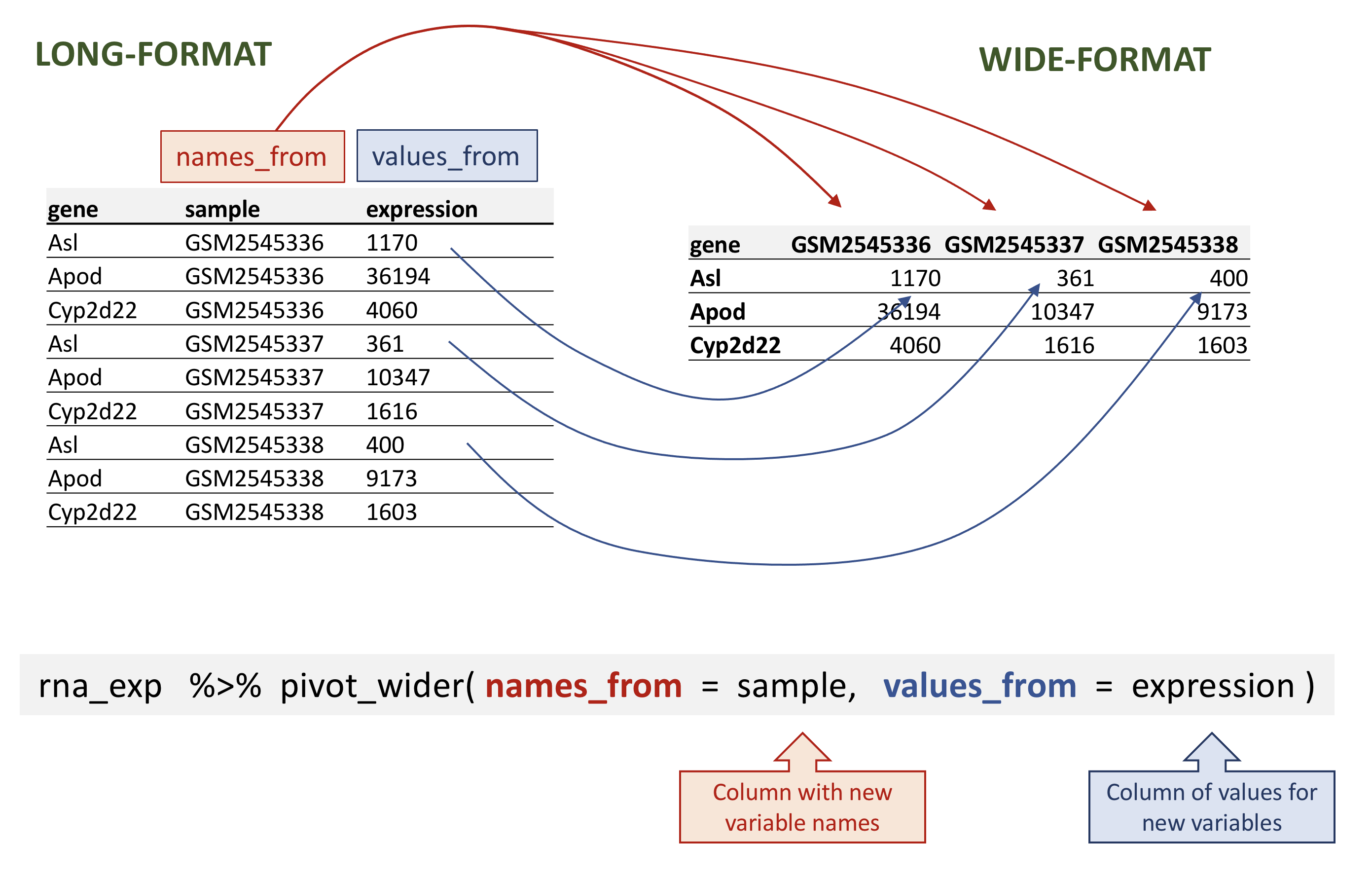
rna data.
R
rna_wide <- rna_exp |>
  pivot_wider(names_from = sample,
              values_from = expression)
rna_wide
OUTPUT
# A tibble: 1,474 × 23
   gene    GSM2545336 GSM2545337 GSM2545338 GSM2545339 GSM2545340 GSM2545341
   <chr>        <dbl>      <dbl>      <dbl>      <dbl>      <dbl>      <dbl>
 1 Asl           1170        361        400        586        626        988
 2 Apod         36194      10347       9173      10620      13021      29594
 3 Cyp2d22       4060       1616       1603       1901       2171       3349
 4 Klk6           287        629        641        578        448        195
 5 Fcrls           85        233        244        237        180         38
 6 Slc2a4         782        231        248        265        313        786
 7 Exd2          1619       2288       2235       2513       2366       1359
 8 Gjc2           288        595        568        551        310        146
 9 Plp1         43217     101241      96534      58354      53126      27173
10 Gnb4          1071       1791       1867       1430       1355        798
# ℹ 1,464 more rows
# ℹ 16 more variables: GSM2545342 <dbl>, GSM2545343 <dbl>, GSM2545344 <dbl>,
#   GSM2545345 <dbl>, GSM2545346 <dbl>, GSM2545347 <dbl>, GSM2545348 <dbl>,
#   GSM2545349 <dbl>, GSM2545350 <dbl>, GSM2545351 <dbl>, GSM2545352 <dbl>,
#   GSM2545353 <dbl>, GSM2545354 <dbl>, GSM2545362 <dbl>, GSM2545363 <dbl>,
#   GSM2545380 <dbl>
Note that by default, the pivot_wider() function will
add NA for missing values.
Let’s imagine that for some reason, we had some missing expression values for some genes in certain samples. In the following fictive example, the gene Cyp2d22 has only one expression value, in GSM2545338 sample.
R
rna_with_missing_values <- rna |>
  select(gene, sample, expression) |>
  filter(gene %in% c("Asl", "Apod", "Cyp2d22")) |>
  filter(sample %in% c("GSM2545336", "GSM2545337", "GSM2545338")) |>
  arrange(sample) |>
  filter(!(gene == "Cyp2d22" & sample != "GSM2545338"))
rna_with_missing_values
OUTPUT
# A tibble: 7 × 3
  gene    sample     expression
  <chr>   <chr>           <dbl>
1 Asl     GSM2545336       1170
2 Apod    GSM2545336      36194
3 Asl     GSM2545337        361
4 Apod    GSM2545337      10347
5 Asl     GSM2545338        400
6 Apod    GSM2545338       9173
7 Cyp2d22 GSM2545338       1603
By default, the pivot_wider() function will add
NA for missing values. This can be parameterised with the
values_fill argument of the pivot_wider()
function.
R
rna_with_missing_values |>
  pivot_wider(names_from = sample,
              values_from = expression)
OUTPUT
# A tibble: 3 × 4
  gene    GSM2545336 GSM2545337 GSM2545338
  <chr>        <dbl>      <dbl>      <dbl>
1 Asl           1170        361        400
2 Apod         36194      10347       9173
3 Cyp2d22         NA         NA       1603
R
rna_with_missing_values |>
  pivot_wider(names_from = sample,
              values_from = expression,
              values_fill = 0)
OUTPUT
# A tibble: 3 × 4
  gene    GSM2545336 GSM2545337 GSM2545338
  <chr>        <dbl>      <dbl>      <dbl>
1 Asl           1170        361        400
2 Apod         36194      10347       9173
3 Cyp2d22          0          0       1603
Pivoting data into a longer format
In the opposite situation we are using the column names and turning them into a pair of new variables. One variable represents the column names as values, and the other variable contains the values previously associated with the column names.
pivot_longer() takes four main arguments:
- the data to be transformed;
- the
names_to: the new column name we wish to create and populate with the current column names; - the
values_to: the new column name we wish to create and populate with current values; - the names of the columns to be used to populate the
names_toandvalues_tovariables (or to drop).
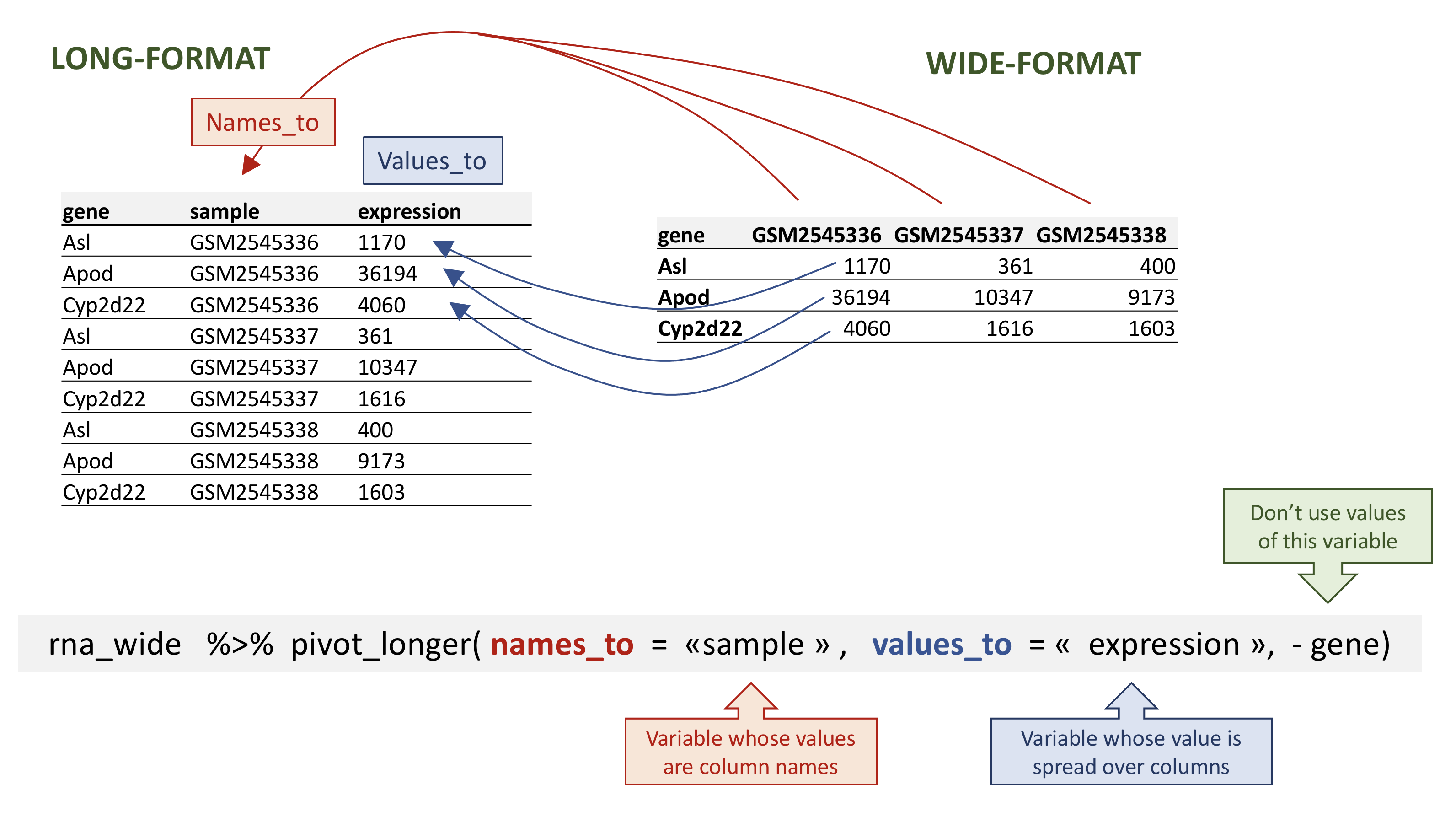
rna data.
To recreate rna_long from rna_wide we would
create a key called sample and value called
expression and use all columns except gene for
the key variable. Here we drop gene column with a minus
sign.
Notice how the new variable names are to be quoted here.
R
rna_long <- rna_wide |>
    pivot_longer(names_to = "sample",
                 values_to = "expression",
                 -gene)
rna_long
OUTPUT
# A tibble: 32,428 × 3
   gene  sample     expression
   <chr> <chr>           <dbl>
 1 Asl   GSM2545336       1170
 2 Asl   GSM2545337        361
 3 Asl   GSM2545338        400
 4 Asl   GSM2545339        586
 5 Asl   GSM2545340        626
 6 Asl   GSM2545341        988
 7 Asl   GSM2545342        836
 8 Asl   GSM2545343        535
 9 Asl   GSM2545344        586
10 Asl   GSM2545345        597
# ℹ 32,418 more rows
We could also have used a specification for what columns to include.
This can be useful if you have a large number of identifying columns,
and it’s easier to specify what to gather than what to leave alone. Here
the starts_with() function can help to retrieve sample
names without having to list them all! Another possibility would be to
use the : operator!
R
rna_wide |>
    pivot_longer(names_to = "sample",
                 values_to = "expression",
                 cols = starts_with("GSM"))
OUTPUT
# A tibble: 32,428 × 3
   gene  sample     expression
   <chr> <chr>           <dbl>
 1 Asl   GSM2545336       1170
 2 Asl   GSM2545337        361
 3 Asl   GSM2545338        400
 4 Asl   GSM2545339        586
 5 Asl   GSM2545340        626
 6 Asl   GSM2545341        988
 7 Asl   GSM2545342        836
 8 Asl   GSM2545343        535
 9 Asl   GSM2545344        586
10 Asl   GSM2545345        597
# ℹ 32,418 more rows
R
rna_wide |>
    pivot_longer(names_to = "sample",
                 values_to = "expression",
                 GSM2545336:GSM2545380)
OUTPUT
# A tibble: 32,428 × 3
   gene  sample     expression
   <chr> <chr>           <dbl>
 1 Asl   GSM2545336       1170
 2 Asl   GSM2545337        361
 3 Asl   GSM2545338        400
 4 Asl   GSM2545339        586
 5 Asl   GSM2545340        626
 6 Asl   GSM2545341        988
 7 Asl   GSM2545342        836
 8 Asl   GSM2545343        535
 9 Asl   GSM2545344        586
10 Asl   GSM2545345        597
# ℹ 32,418 more rows
Note that if we had missing values in the wide-format, the
NA would be included in the new long format.
Remember our previous fictive tibble containing missing values:
R
rna_with_missing_values
OUTPUT
# A tibble: 7 × 3
  gene    sample     expression
  <chr>   <chr>           <dbl>
1 Asl     GSM2545336       1170
2 Apod    GSM2545336      36194
3 Asl     GSM2545337        361
4 Apod    GSM2545337      10347
5 Asl     GSM2545338        400
6 Apod    GSM2545338       9173
7 Cyp2d22 GSM2545338       1603
R
wide_with_NA <- rna_with_missing_values |>
  pivot_wider(names_from = sample,
              values_from = expression)
wide_with_NA
OUTPUT
# A tibble: 3 × 4
  gene    GSM2545336 GSM2545337 GSM2545338
  <chr>        <dbl>      <dbl>      <dbl>
1 Asl           1170        361        400
2 Apod         36194      10347       9173
3 Cyp2d22         NA         NA       1603
R
wide_with_NA |>
    pivot_longer(names_to = "sample",
                 values_to = "expression",
                 -gene)
OUTPUT
# A tibble: 9 × 3
  gene    sample     expression
  <chr>   <chr>           <dbl>
1 Asl     GSM2545336       1170
2 Asl     GSM2545337        361
3 Asl     GSM2545338        400
4 Apod    GSM2545336      36194
5 Apod    GSM2545337      10347
6 Apod    GSM2545338       9173
7 Cyp2d22 GSM2545336         NA
8 Cyp2d22 GSM2545337         NA
9 Cyp2d22 GSM2545338       1603
Pivoting to wider and longer formats can be a useful way to balance out a dataset so every replicate has the same composition.
Question
Starting from the rna table, use the pivot_wider()
function to create a wide-format table giving the gene expression levels
in each mouse. Then use the pivot_longer() function to
restore a long-format table.
R
rna1 <- rna |>
select(gene, mouse, expression) |>
pivot_wider(names_from = mouse, values_from = expression)
rna1
OUTPUT
# A tibble: 1,474 × 23
   gene     `14`    `9`  `10`  `15`  `18`   `6`   `5`  `11`  `22`  `13`  `23`
   <chr>   <dbl>  <dbl> <dbl> <dbl> <dbl> <dbl> <dbl> <dbl> <dbl> <dbl> <dbl>
 1 Asl      1170    361   400   586   626   988   836   535   586   597   938
 2 Apod    36194  10347  9173 10620 13021 29594 24959 13668 13230 15868 27769
 3 Cyp2d22  4060   1616  1603  1901  2171  3349  3122  2008  2254  2277  2985
 4 Klk6      287    629   641   578   448   195   186  1101   537   567   327
 5 Fcrls      85    233   244   237   180    38    68   375   199   177    89
 6 Slc2a4    782    231   248   265   313   786   528   249   266   357   654
 7 Exd2     1619   2288  2235  2513  2366  1359  1474  3126  2379  2173  1531
 8 Gjc2      288    595   568   551   310   146   186   791   454   370   240
 9 Plp1    43217 101241 96534 58354 53126 27173 28728 98658 61356 61647 38019
10 Gnb4     1071   1791  1867  1430  1355   798   806  2437  1394  1554   960
# ℹ 1,464 more rows
# ℹ 11 more variables: `24` <dbl>, `8` <dbl>, `7` <dbl>, `1` <dbl>, `16` <dbl>,
#   `21` <dbl>, `4` <dbl>, `2` <dbl>, `20` <dbl>, `12` <dbl>, `19` <dbl>
R
rna1 |>
pivot_longer(names_to = "mouse_id", values_to = "counts", -gene)
OUTPUT
# A tibble: 32,428 × 3
   gene  mouse_id counts
   <chr> <chr>     <dbl>
 1 Asl   14         1170
 2 Asl   9           361
 3 Asl   10          400
 4 Asl   15          586
 5 Asl   18          626
 6 Asl   6           988
 7 Asl   5           836
 8 Asl   11          535
 9 Asl   22          586
10 Asl   13          597
# ℹ 32,418 more rowsQuestion
Subset genes located on X and Y chromosomes from the rna
data frame and spread the data frame with sex as columns,
chromosome_name as rows, and the mean expression of genes
located in each chromosome as the values, as in the following
tibble:
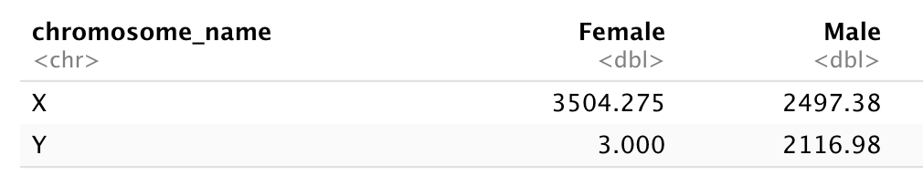
You will need to summarise before reshaping!
Let’s first calculate the mean expression level of X and Y linked genes from male and female samples…
R
 rna |>
  filter(chromosome_name == "Y" | chromosome_name == "X") |>
  group_by(sex, chromosome_name) |>
  summarise(mean = mean(expression))
OUTPUT
`summarise()` has regrouped the output.
ℹ Summaries were computed grouped by sex and chromosome_name.
ℹ Output is grouped by sex.
ℹ Use `summarise(.groups = "drop_last")` to silence this message.
ℹ Use `summarise(.by = c(sex, chromosome_name))` for per-operation grouping
  (`?dplyr::dplyr_by`) instead.
OUTPUT
# A tibble: 4 × 3
# Groups:   sex [2]
  sex    chromosome_name  mean
  <chr>  <chr>           <dbl>
1 Female X               3504.
2 Female Y                  3
3 Male   X               2497.
4 Male   Y               2117.
And pivot the table to wide format
R
rna_1 <- rna |>
  filter(chromosome_name == "Y" | chromosome_name == "X") |>
  group_by(sex, chromosome_name) |>
  summarise(mean = mean(expression)) |>
  pivot_wider(names_from = sex,
              values_from = mean)
OUTPUT
`summarise()` has regrouped the output.
ℹ Summaries were computed grouped by sex and chromosome_name.
ℹ Output is grouped by sex.
ℹ Use `summarise(.groups = "drop_last")` to silence this message.
ℹ Use `summarise(.by = c(sex, chromosome_name))` for per-operation grouping
  (`?dplyr::dplyr_by`) instead.
R
rna_1
OUTPUT
# A tibble: 2 × 3
  chromosome_name Female  Male
  <chr>            <dbl> <dbl>
1 X                3504. 2497.
2 Y                   3  2117.
Now take that data frame and transform it with
pivot_longer() so each row is a unique
chromosome_name by gender combination.
R
rna_1 |>
  pivot_longer(names_to = "gender",
               values_to = "mean",
               -chromosome_name)
OUTPUT
# A tibble: 4 × 3
  chromosome_name gender  mean
  <chr>           <chr>  <dbl>
1 X               Female 3504.
2 X               Male   2497.
3 Y               Female    3
4 Y Male 2117.Question
Use the rna dataset to create an expression matrix where
each row represents the mean expression levels of genes and columns
represent the different timepoints.
Let’s first calculate the mean expression by gene and by time
R
rna |>
  group_by(gene, time) |>
  summarise(mean_exp = mean(expression))
OUTPUT
`summarise()` has regrouped the output.
ℹ Summaries were computed grouped by gene and time.
ℹ Output is grouped by gene.
ℹ Use `summarise(.groups = "drop_last")` to silence this message.
ℹ Use `summarise(.by = c(gene, time))` for per-operation grouping
  (`?dplyr::dplyr_by`) instead.
OUTPUT
# A tibble: 4,422 × 3
# Groups:   gene [1,474]
   gene      time mean_exp
   <chr>    <dbl>    <dbl>
 1 AI504432     0    1034.
 2 AI504432     4    1104.
 3 AI504432     8    1014
 4 AW046200     0     155.
 5 AW046200     4     152.
 6 AW046200     8      81
 7 AW551984     0     238
 8 AW551984     4     302.
 9 AW551984     8     342.
10 Aamp         0    4603.
# ℹ 4,412 more rows
before using the pivot_wider() function
R
rna_time <- rna |>
  group_by(gene, time) |>
  summarise(mean_exp = mean(expression)) |>
  pivot_wider(names_from = time,
              values_from = mean_exp)
OUTPUT
`summarise()` has regrouped the output.
ℹ Summaries were computed grouped by gene and time.
ℹ Output is grouped by gene.
ℹ Use `summarise(.groups = "drop_last")` to silence this message.
ℹ Use `summarise(.by = c(gene, time))` for per-operation grouping
  (`?dplyr::dplyr_by`) instead.
R
rna_time
OUTPUT
# A tibble: 1,474 × 4
# Groups:   gene [1,474]
   gene         `0`     `4`     `8`
   <chr>      <dbl>   <dbl>   <dbl>
 1 AI504432 1034.   1104.   1014
 2 AW046200  155.    152.     81
 3 AW551984  238     302.    342.
 4 Aamp     4603.   4870    4763.
 5 Abca12      5.29    4.25    4.14
 6 Abcc8    2576.   2609.   2292.
 7 Abhd14a   591.    547.    432.
 8 Abi2     4881.   4903.   4945.
 9 Abi3bp   1175.   1061.    762.
10 Abl2     2170.   2078.   2131.
# ℹ 1,464 more rows
Notice that this generates a tibble with some column names starting by a number. If we wanted to select the column corresponding to the timepoints, we could not use the column names directly… What happens when we select the column 4?
R
rna |>
  group_by(gene, time) |>
  summarise(mean_exp = mean(expression)) |>
  pivot_wider(names_from = time,
              values_from = mean_exp) |>
  select(gene, 4)
OUTPUT
`summarise()` has regrouped the output.
ℹ Summaries were computed grouped by gene and time.
ℹ Output is grouped by gene.
ℹ Use `summarise(.groups = "drop_last")` to silence this message.
ℹ Use `summarise(.by = c(gene, time))` for per-operation grouping
  (`?dplyr::dplyr_by`) instead.
OUTPUT
# A tibble: 1,474 × 2
# Groups:   gene [1,474]
   gene         `8`
   <chr>      <dbl>
 1 AI504432 1014
 2 AW046200   81
 3 AW551984  342.
 4 Aamp     4763.
 5 Abca12      4.14
 6 Abcc8    2292.
 7 Abhd14a   432.
 8 Abi2     4945.
 9 Abi3bp    762.
10 Abl2     2131.
# ℹ 1,464 more rows
To select the timepoint 4, we would have to quote the column name, with backticks “`”
R
rna |>
  group_by(gene, time) |>
  summarise(mean_exp = mean(expression)) |>
  pivot_wider(names_from = time,
              values_from = mean_exp) |>
  select(gene, `4`)
OUTPUT
`summarise()` has regrouped the output.
ℹ Summaries were computed grouped by gene and time.
ℹ Output is grouped by gene.
ℹ Use `summarise(.groups = "drop_last")` to silence this message.
ℹ Use `summarise(.by = c(gene, time))` for per-operation grouping
  (`?dplyr::dplyr_by`) instead.
OUTPUT
# A tibble: 1,474 × 2
# Groups:   gene [1,474]
   gene         `4`
   <chr>      <dbl>
 1 AI504432 1104.
 2 AW046200  152.
 3 AW551984  302.
 4 Aamp     4870
 5 Abca12      4.25
 6 Abcc8    2609.
 7 Abhd14a   547.
 8 Abi2     4903.
 9 Abi3bp   1061.
10 Abl2     2078.
# ℹ 1,464 more rows
Another possibility would be to rename the column, choosing a name that doesn’t start by a number :
R
rna |>
  group_by(gene, time) |>
  summarise(mean_exp = mean(expression)) |>
  pivot_wider(names_from = time,
              values_from = mean_exp) |>
  rename("time0" = `0`, "time4" = `4`, "time8" = `8`) |>
  select(gene, time4)
OUTPUT
`summarise()` has regrouped the output.
ℹ Summaries were computed grouped by gene and time.
ℹ Output is grouped by gene.
ℹ Use `summarise(.groups = "drop_last")` to silence this message.
ℹ Use `summarise(.by = c(gene, time))` for per-operation grouping
  (`?dplyr::dplyr_by`) instead.
OUTPUT
# A tibble: 1,474 × 2
# Groups:   gene [1,474]
   gene       time4
   <chr>      <dbl>
 1 AI504432 1104.
 2 AW046200  152.
 3 AW551984  302.
 4 Aamp     4870
 5 Abca12      4.25
 6 Abcc8    2609.
 7 Abhd14a   547.
 8 Abi2     4903.
 9 Abi3bp   1061.
10 Abl2     2078.
# ℹ 1,464 more rowsQuestion
Use the previous data frame containing mean expression levels per timepoint and create a new column containing fold-changes between timepoint 8 and timepoint 0, and fold-changes between timepoint 8 and timepoint 4. Convert this table into a long-format table gathering the fold-changes calculated.
Starting from the rna_time tibble:
R
rna_time
OUTPUT
# A tibble: 1,474 × 4
# Groups:   gene [1,474]
   gene         `0`     `4`     `8`
   <chr>      <dbl>   <dbl>   <dbl>
 1 AI504432 1034.   1104.   1014
 2 AW046200  155.    152.     81
 3 AW551984  238     302.    342.
 4 Aamp     4603.   4870    4763.
 5 Abca12      5.29    4.25    4.14
 6 Abcc8    2576.   2609.   2292.
 7 Abhd14a   591.    547.    432.
 8 Abi2     4881.   4903.   4945.
 9 Abi3bp   1175.   1061.    762.
10 Abl2     2170.   2078.   2131.
# ℹ 1,464 more rows
Calculate fold-changes:
R
rna_time |>
  mutate(time_8_vs_0 = `8` / `0`, time_8_vs_4 = `8` / `4`)
OUTPUT
# A tibble: 1,474 × 6
# Groups:   gene [1,474]
   gene         `0`     `4`     `8` time_8_vs_0 time_8_vs_4
   <chr>      <dbl>   <dbl>   <dbl>       <dbl>       <dbl>
 1 AI504432 1034.   1104.   1014          0.981       0.918
 2 AW046200  155.    152.     81          0.522       0.532
 3 AW551984  238     302.    342.         1.44        1.13
 4 Aamp     4603.   4870    4763.         1.03        0.978
 5 Abca12      5.29    4.25    4.14       0.784       0.975
 6 Abcc8    2576.   2609.   2292.         0.889       0.878
 7 Abhd14a   591.    547.    432.         0.731       0.791
 8 Abi2     4881.   4903.   4945.         1.01        1.01
 9 Abi3bp   1175.   1061.    762.         0.649       0.719
10 Abl2     2170.   2078.   2131.         0.982       1.03
# ℹ 1,464 more rows
And use the pivot_longer() function:
R
rna_time |>
  mutate(time_8_vs_0 = `8` / `0`, time_8_vs_4 = `8` / `4`) |>
  pivot_longer(names_to = "comparisons",
               values_to = "Fold_changes",
               time_8_vs_0:time_8_vs_4)
OUTPUT
# A tibble: 2,948 × 6
# Groups:   gene [1,474]
   gene         `0`     `4`     `8` comparisons Fold_changes
   <chr>      <dbl>   <dbl>   <dbl> <chr>              <dbl>
 1 AI504432 1034.   1104.   1014    time_8_vs_0        0.981
 2 AI504432 1034.   1104.   1014    time_8_vs_4        0.918
 3 AW046200  155.    152.     81    time_8_vs_0        0.522
 4 AW046200  155.    152.     81    time_8_vs_4        0.532
 5 AW551984  238     302.    342.   time_8_vs_0        1.44
 6 AW551984  238     302.    342.   time_8_vs_4        1.13
 7 Aamp     4603.   4870    4763.   time_8_vs_0        1.03
 8 Aamp     4603.   4870    4763.   time_8_vs_4        0.978
 9 Abca12      5.29    4.25    4.14 time_8_vs_0        0.784
10 Abca12      5.29    4.25    4.14 time_8_vs_4        0.975
# ℹ 2,938 more rows
Joining tables
In many real life situations, data are spread across multiple tables. Usually this occurs because different types of information are collected from different sources.
It may be desirable for some analyses to combine data from two or more tables into a single data frame based on a column that would be common to all the tables.
The dplyr package provides a set of join functions for
combining two data frames based on matches within specified columns.
Here, we provide a short introduction to joins. For further reading,
please refer to the chapter about table
joins. The Data
Transformation Cheat Sheet also provides a short overview on table
joins.
We are going to illustrate join using a small table,
rna_mini that we will create by subsetting the original
rna table, keeping only 3 columns and 10 lines.
R
rna_mini <- rna |>
   select(gene, sample, expression) |>
   head(10)
rna_mini
OUTPUT
# A tibble: 10 × 3
   gene    sample     expression
   <chr>   <chr>           <dbl>
 1 Asl     GSM2545336       1170
 2 Apod    GSM2545336      36194
 3 Cyp2d22 GSM2545336       4060
 4 Klk6    GSM2545336        287
 5 Fcrls   GSM2545336         85
 6 Slc2a4  GSM2545336        782
 7 Exd2    GSM2545336       1619
 8 Gjc2    GSM2545336        288
 9 Plp1    GSM2545336      43217
10 Gnb4    GSM2545336       1071
The second table, annot1, contains 2 columns, gene and
gene_description. You can either download
annot1.csv by clicking on the link and then moving it to the
data/ folder, or you can use the R code below to download
it directly to the folder.
R
download.file(url = "https://carpentries-incubator.github.io/bioc-intro/data/annot1.csv",
              destfile = "data/annot1.csv")
annot1 <- read_csv(file = "data/annot1.csv")
annot1
OUTPUT
# A tibble: 10 × 2
   gene    gene_description
   <chr>   <chr>
 1 Cyp2d22 cytochrome P450, family 2, subfamily d, polypeptide 22 [Source:MGI S…
 2 Klk6    kallikrein related-peptidase 6 [Source:MGI Symbol;Acc:MGI:1343166]
 3 Fcrls   Fc receptor-like S, scavenger receptor [Source:MGI Symbol;Acc:MGI:19…
 4 Plp1    proteolipid protein (myelin) 1 [Source:MGI Symbol;Acc:MGI:97623]
 5 Exd2    exonuclease 3'-5' domain containing 2 [Source:MGI Symbol;Acc:MGI:192…
 6 Apod    apolipoprotein D [Source:MGI Symbol;Acc:MGI:88056]
 7 Gnb4    guanine nucleotide binding protein (G protein), beta 4 [Source:MGI S…
 8 Slc2a4  solute carrier family 2 (facilitated glucose transporter), member 4 …
 9 Asl     argininosuccinate lyase [Source:MGI Symbol;Acc:MGI:88084]
10 Gjc2    gap junction protein, gamma 2 [Source:MGI Symbol;Acc:MGI:2153060]
We now want to join these two tables into a single one containing all
variables using the full_join() function from the
dplyr package. The function will automatically find the
common variable to match columns from the first and second table. In
this case, gene is the common variable. Such variables are
called keys. Keys are used to match observations across different
tables.
R
full_join(rna_mini, annot1)
OUTPUT
Joining with `by = join_by(gene)`OUTPUT
# A tibble: 10 × 4
   gene    sample     expression gene_description
   <chr>   <chr>           <dbl> <chr>
 1 Asl     GSM2545336       1170 argininosuccinate lyase [Source:MGI Symbol;Acc…
 2 Apod    GSM2545336      36194 apolipoprotein D [Source:MGI Symbol;Acc:MGI:88…
 3 Cyp2d22 GSM2545336       4060 cytochrome P450, family 2, subfamily d, polype…
 4 Klk6    GSM2545336        287 kallikrein related-peptidase 6 [Source:MGI Sym…
 5 Fcrls   GSM2545336         85 Fc receptor-like S, scavenger receptor [Source…
 6 Slc2a4  GSM2545336        782 solute carrier family 2 (facilitated glucose t…
 7 Exd2    GSM2545336       1619 exonuclease 3'-5' domain containing 2 [Source:…
 8 Gjc2    GSM2545336        288 gap junction protein, gamma 2 [Source:MGI Symb…
 9 Plp1    GSM2545336      43217 proteolipid protein (myelin) 1 [Source:MGI Sym…
10 Gnb4    GSM2545336       1071 guanine nucleotide binding protein (G protein)…
In real life, gene annotations are sometimes labelled differently.
The annot2 table is exactly the same than
annot1 except that the variable containing gene names is
labelled differently. Again, either download
annot2.csv yourself and move it to data/ or use the R
code below.
R
download.file(url = "https://carpentries-incubator.github.io/bioc-intro/data/annot2.csv",
              destfile = "data/annot2.csv")
annot2 <- read_csv(file = "data/annot2.csv")
annot2
OUTPUT
# A tibble: 10 × 2
   external_gene_name description
   <chr>              <chr>
 1 Cyp2d22            cytochrome P450, family 2, subfamily d, polypeptide 22 [S…
 2 Klk6               kallikrein related-peptidase 6 [Source:MGI Symbol;Acc:MGI…
 3 Fcrls              Fc receptor-like S, scavenger receptor [Source:MGI Symbol…
 4 Plp1               proteolipid protein (myelin) 1 [Source:MGI Symbol;Acc:MGI…
 5 Exd2               exonuclease 3'-5' domain containing 2 [Source:MGI Symbol;…
 6 Apod               apolipoprotein D [Source:MGI Symbol;Acc:MGI:88056]
 7 Gnb4               guanine nucleotide binding protein (G protein), beta 4 [S…
 8 Slc2a4             solute carrier family 2 (facilitated glucose transporter)…
 9 Asl                argininosuccinate lyase [Source:MGI Symbol;Acc:MGI:88084]
10 Gjc2               gap junction protein, gamma 2 [Source:MGI Symbol;Acc:MGI:…
In case none of the variable names match, we can set manually the
variables to use for the matching. These variables can be set using the
by argument, as shown below with rna_mini and
annot2 tables.
R
full_join(rna_mini, annot2, by = c("gene" = "external_gene_name"))
OUTPUT
# A tibble: 10 × 4
   gene    sample     expression description
   <chr>   <chr>           <dbl> <chr>
 1 Asl     GSM2545336       1170 argininosuccinate lyase [Source:MGI Symbol;Acc…
 2 Apod    GSM2545336      36194 apolipoprotein D [Source:MGI Symbol;Acc:MGI:88…
 3 Cyp2d22 GSM2545336       4060 cytochrome P450, family 2, subfamily d, polype…
 4 Klk6    GSM2545336        287 kallikrein related-peptidase 6 [Source:MGI Sym…
 5 Fcrls   GSM2545336         85 Fc receptor-like S, scavenger receptor [Source…
 6 Slc2a4  GSM2545336        782 solute carrier family 2 (facilitated glucose t…
 7 Exd2    GSM2545336       1619 exonuclease 3'-5' domain containing 2 [Source:…
 8 Gjc2    GSM2545336        288 gap junction protein, gamma 2 [Source:MGI Symb…
 9 Plp1    GSM2545336      43217 proteolipid protein (myelin) 1 [Source:MGI Sym…
10 Gnb4    GSM2545336       1071 guanine nucleotide binding protein (G protein)…
As can be seen above, the variable name of the first table is retained in the joined one.
Challenge:
Download the annot3 table by clicking
this link and put the table in your data/ repository. Using the
full_join() function, join tables rna_mini and
annot3. What has happened for genes Klk6,
mt-Tf, mt-Rnr1, mt-Tv, mt-Rnr2, and
mt-Tl1 ?
R
annot3 <- read_csv("data/annot3.csv")
full_join(rna_mini, annot3)
OUTPUT
# A tibble: 15 × 4
   gene    sample     expression gene_description
   <chr>   <chr>           <dbl> <chr>
 1 Asl     GSM2545336       1170 argininosuccinate lyase [Source:MGI Symbol;Acc…
 2 Apod    GSM2545336      36194 apolipoprotein D [Source:MGI Symbol;Acc:MGI:88…
 3 Cyp2d22 GSM2545336       4060 cytochrome P450, family 2, subfamily d, polype…
 4 Klk6    GSM2545336        287 <NA>
 5 Fcrls   GSM2545336         85 Fc receptor-like S, scavenger receptor [Source…
 6 Slc2a4  GSM2545336        782 solute carrier family 2 (facilitated glucose t…
 7 Exd2    GSM2545336       1619 exonuclease 3'-5' domain containing 2 [Source:…
 8 Gjc2    GSM2545336        288 gap junction protein, gamma 2 [Source:MGI Symb…
 9 Plp1    GSM2545336      43217 proteolipid protein (myelin) 1 [Source:MGI Sym…
10 Gnb4    GSM2545336       1071 guanine nucleotide binding protein (G protein)…
11 mt-Tf   <NA>               NA mitochondrially encoded tRNA phenylalanine [So…
12 mt-Rnr1 <NA>               NA mitochondrially encoded 12S rRNA [Source:MGI S…
13 mt-Tv   <NA>               NA mitochondrially encoded tRNA valine [Source:MG…
14 mt-Rnr2 <NA>               NA mitochondrially encoded 16S rRNA [Source:MGI S…
15 mt-Tl1  <NA>               NA mitochondrially encoded tRNA leucine 1 [Source…
Genes Klk6 is only present in rna_mini, while
genes mt-Tf, mt-Rnr1, mt-Tv,
mt-Rnr2, and mt-Tl1 are only present in
annot3 table. Their respective values for the variables of
the table have been encoded as missing.
Exporting data
Now that you have learned how to use dplyr to extract
information from or summarise your raw data, you may want to export
these new data sets to share them with your collaborators or for
archival.
Similar to the read_csv() function used for reading CSV
files into R, there is a write_csv() function that
generates CSV files from data frames.
Before using write_csv(), we are going to create a new
folder, data_output, in our working directory that will
store this generated dataset. We don’t want to write generated datasets
in the same directory as our raw data. It’s good practice to keep them
separate. The data folder should only contain the raw,
unaltered data, and should be left alone to make sure we don’t delete or
modify it. In contrast, our script will generate the contents of the
data_output directory, so even if the files it contains are
deleted, we can always re-generate them.
Let’s use write_csv() to save the rna_wide table that we
have created previously.
R
write_csv(rna_wide, file = "data_output/rna_wide.csv")
- Tabular data in R using the tidyverse meta-package