Introduction to R
Last updated on 2026-04-21 | Edit this page
Overview
Questions
- First commands in R
Objectives
- Define the following terms as they relate to R: object, assign, call, function, arguments, options.
- Assign values to objects in R.
- Learn how to name objects
- Use comments to inform script.
- Solve simple arithmetic operations in R.
- Call functions and use arguments to change their default options.
- Inspect the content of vectors and manipulate their content.
- Subset and extract values from vectors.
- Analyze vectors with missing data.
This episode is based on the Data Carpentries’s Data Analysis and Visualisation in R for Ecologists lesson.
Creating objects in R
You can get output from R simply by typing math in the console:
R
3 + 5
OUTPUT
[1] 8R
12 / 7
OUTPUT
[1] 1.714286However, to do useful and interesting things, we need to assign
values to objects. To create an object, we need to
give it a name followed by the assignment operator <-,
and the value we want to give it:
R
weight_kg <- 55
<- is the assignment operator. It assigns values on
the right to objects on the left. So, after executing
x <- 3, the value of x is 3.
The arrow can be read as 3 goes into x.
For historical reasons, you can also use = for assignments,
but not in every context. Because of the slight
differences in syntax, it is good practice to always use
<- for assignments.
In RStudio, typing Alt + - (push Alt
at the same time as the - key) will write <-
in a single keystroke in a PC, while typing Option +
- (push Option at the same time as the
- key) does the same in a Mac.
Naming variables
Objects can be given any name such as x,
current_temperature, or subject_id. You want
your object names to be explicit and not too long. They cannot start
with a number (2x is not valid, but x2 is). R
is case sensitive (e.g., weight_kg is different from
Weight_kg). There are some names that cannot be used
because they are the names of fundamental functions in R (e.g.,
if, else, for, see the Reserved
Words in R manual page, for a complete list). In general, even if
it’s allowed, it’s best to not use other function names (e.g.,
c, T, mean, data,
df, weights). If in doubt, check the help to
see if the name is already in use. It’s also best to avoid dots
(.) within an object name as in my.dataset.
There are many functions in R with dots in their names for historical
reasons, but because dots have a special meaning in R (for methods) and
other programming languages, it’s best to avoid them. It is also
recommended to use nouns for object names, and verbs for function names.
It’s important to be consistent in the styling of your code (where you
put spaces, how you name objects, etc.). Using a consistent coding style
makes your code clearer to read for your future self and your
collaborators. In R, some popular style guides are Google’s, the
tidyverse’s style and the Bioconductor
style guide. The tidyverse’s is very comprehensive and may seem
overwhelming at first. You can install the lintr
package to automatically check for issues in the styling of your
code.
Objects vs. variables: What are known as
objectsinRare known asvariablesin many other programming languages. Depending on the context,objectandvariablecan have drastically different meanings. However, in this lesson, the two words are used synonymously. For more information see here.
When assigning a value to an object, R does not print anything. You can force R to print the value by using parentheses or by typing the object name:
R
weight_kg <- 55    # doesn't print anything
(weight_kg <- 55)  # but putting parenthesis around the call prints the value of `weight_kg`
OUTPUT
[1] 55R
weight_kg # and so does typing the name of the object
OUTPUT
[1] 55Now that R has weight_kg in memory, we can do arithmetic
with it. For instance, we may want to convert this weight into pounds
(weight in pounds is 2.2 times the weight in kg):
R
2.2 * weight_kg
OUTPUT
[1] 121We can also change an object’s value by assigning it a new one:
R
weight_kg <- 57.5
2.2 * weight_kg
OUTPUT
[1] 126.5This means that assigning a value to one object does not change the
values of other objects For example, let’s store the animal’s weight in
pounds in a new object, weight_lb:
R
weight_lb <- 2.2 * weight_kg
and then change weight_kg to 100.
R
weight_kg <- 100
Challenge:
What do you think is the current content of the object
weight_lb? 126.5 or 220?
Comments
The comment character in R is #, anything to the right
of a # in a script will be ignored by R. It is useful to
leave notes, and explanations in your scripts.
RStudio makes it easy to comment or uncomment a paragraph: after selecting the lines you want to comment, press at the same time on your keyboard Ctrl + Shift + C. If you only want to comment out one line, you can put the cursor at any location of that line (i.e. no need to select the whole line), then press Ctrl + Shift + C.
Challenge
What are the values after each statement in the following?
R
mass <- 47.5            # mass?
age  <- 122             # age?
mass <- mass * 2.0      # mass?
age  <- age - 20        # age?
mass_index <- mass/age  # mass_index?
Functions and their arguments
Functions are “canned scripts” that automate more complicated sets of
commands including operations assignments, etc. Many functions are
predefined, or can be made available by importing R packages
(more on that later). A function usually gets one or more inputs called
arguments. Functions often (but not always) return a
value. A typical example would be the function
sqrt(). The input (the argument) must be a number, and the
return value (in fact, the output) is the square root of that number.
Executing a function (‘running it’) is called calling the
function. An example of a function call is:
R
b <- sqrt(a)
Here, the value of a is given to the sqrt()
function, the sqrt() function calculates the square root,
and returns the value which is then assigned to the object
b. This function is very simple, because it takes just one
argument.
The return ‘value’ of a function need not be numerical (like that of
sqrt()), and it also does not need to be a single item: it
can be a set of things, or even a dataset. We’ll see that when we read
data files into R.
Arguments can be anything, not only numbers or filenames, but also other objects. Exactly what each argument means differs per function, and must be looked up in the documentation (see below). Some functions take arguments which may either be specified by the user, or, if left out, take on a default value: these are called options. Options are typically used to alter the way the function operates, such as whether it ignores ‘bad values’, or what symbol to use in a plot. However, if you want something specific, you can specify a value of your choice which will be used instead of the default.
Let’s try a function that can take multiple arguments:
round().
R
round(3.14159)
OUTPUT
[1] 3Here, we’ve called round() with just one argument,
3.14159, and it has returned the value 3.
That’s because the default is to round to the nearest whole number. If
we want more digits we can see how to do that by getting information
about the round function. We can use
args(round) or look at the help for this function using
?round.
R
args(round)
OUTPUT
function (x, digits = 0, ...)
NULL
R
?round
We see that if we want a different number of digits, we can type
digits=2 or however many we want.
R
round(3.14159, digits = 2)
OUTPUT
[1] 3.14If you provide the arguments in the exact same order as they are defined you don’t have to name them:
R
round(3.14159, 2)
OUTPUT
[1] 3.14And if you do name the arguments, you can switch their order:
R
round(digits = 2, x = 3.14159)
OUTPUT
[1] 3.14It’s good practice to put the non-optional arguments (like the number you’re rounding) first in your function call, and to specify the names of all optional arguments. If you don’t, someone reading your code might have to look up the definition of a function with unfamiliar arguments to understand what you’re doing. By specifying the name of the arguments you are also safeguarding against possible future changes in the function interface, which may potentially add new arguments in between the existing ones.
Vectors and data types
A vector is the most common and basic data type in R, and is pretty
much the workhorse of R. A vector is composed by a series of values,
such as numbers or characters. We can assign a series of values to a
vector using the c() function. For example we can create a
vector of animal weights and assign it to a new object
weight_g:
R
weight_g <- c(50, 60, 65, 82)
weight_g
OUTPUT
[1] 50 60 65 82A vector can also contain characters:
R
molecules <- c("dna", "rna", "protein")
molecules
OUTPUT
[1] "dna" "rna" "protein"The quotes around “dna”, “rna”, etc. are essential here. Without the
quotes R will assume there are objects called dna,
rna and protein. As these objects don’t exist
in R’s memory, there will be an error message.
There are many functions that allow you to inspect the content of a
vector. length() tells you how many elements are in a
particular vector:
R
length(weight_g)
OUTPUT
[1] 4R
length(molecules)
OUTPUT
[1] 3An important feature of a vector, is that all of the elements are the
same type of data. The function class() indicates the class
(the type of element) of an object:
R
class(weight_g)
OUTPUT
[1] "numeric"R
class(molecules)
OUTPUT
[1] "character"The function str() provides an overview of the structure
of an object and its elements. It is a useful function when working with
large and complex objects:
R
str(weight_g)
OUTPUT
num [1:4] 50 60 65 82R
str(molecules)
OUTPUT
chr [1:3] "dna" "rna" "protein"You can use the c() function to add other elements to
your vector:
R
weight_g <- c(weight_g, 90) # add to the end of the vector
weight_g <- c(30, weight_g) # add to the beginning of the vector
weight_g
OUTPUT
[1] 30 50 60 65 82 90In the first line, we take the original vector weight_g,
add the value 90 to the end of it, and save the result back
into weight_g. Then we add the value 30 to the
beginning, again saving the result back into weight_g.
We can do this over and over again to grow a vector, or assemble a dataset. As we program, this may be useful to add results that we are collecting or calculating.
An atomic vector is the simplest R data
type and is a linear vector of a single type. Above, we saw 2
of the 6 main atomic vector types that R uses:
"character" and "numeric" (or
"double"). These are the basic building blocks that all R
objects are built from. The other 4 atomic vector types
are:
-
"logical"forTRUEandFALSE(the boolean data type) -
"integer"for integer numbers (e.g.,2L, theLindicates to R that it’s an integer) -
"complex"to represent complex numbers with real and imaginary parts (e.g.,1 + 4i) and that’s all we’re going to say about them -
"raw"for bitstreams that we won’t discuss further
You can check the type of your vector using the typeof()
function and inputting your vector as the argument.
Vectors are one of the many data structures that R
uses. Other important ones are lists (list), matrices
(matrix), data frames (data.frame), factors
(factor) and arrays (array).
Challenge:
We’ve seen that atomic vectors can be of type character, numeric (or double), integer, and logical. But what happens if we try to mix these types in a single vector?
R implicitly converts them to all be the same type
Challenge:
What will happen in each of these examples? (hint: use
class() to check the data type of your objects and type in
their names to see what happens):
R
num_char <- c(1, 2, 3, "a")
num_logical <- c(1, 2, 3, TRUE, FALSE)
char_logical <- c("a", "b", "c", TRUE)
tricky <- c(1, 2, 3, "4")
R
class(num_char)
OUTPUT
[1] "character"R
num_char
OUTPUT
[1] "1" "2" "3" "a"R
class(num_logical)
OUTPUT
[1] "numeric"R
num_logical
OUTPUT
[1] 1 2 3 1 0R
class(char_logical)
OUTPUT
[1] "character"R
char_logical
OUTPUT
[1] "a" "b" "c" "TRUE"R
class(tricky)
OUTPUT
[1] "character"R
tricky
OUTPUT
[1] "1" "2" "3" "4"Challenge:
Why do you think it happens?
Vectors can be of only one data type. R tries to convert (coerce) the content of this vector to find a common denominator that doesn’t lose any information.
Challenge:
How many values in combined_logical are
"TRUE" (as a character) in the following example:
R
num_logical <- c(1, 2, 3, TRUE)
char_logical <- c("a", "b", "c", TRUE)
combined_logical <- c(num_logical, char_logical)
Only one. There is no memory of past data types, and the coercion
happens the first time the vector is evaluated. Therefore, the
TRUE in num_logical gets converted into a
1 before it gets converted into "1" in
combined_logical.
R
combined_logical
OUTPUT
[1] "1" "2" "3" "1" "a" "b" "c" "TRUE"Challenge:
In R, we call converting objects from one class into another class coercion. These conversions happen according to a hierarchy, whereby some types get preferentially coerced into other types. Can you draw a diagram that represents the hierarchy of how these data types are coerced?
logical → numeric → character ← logical
Subsetting vectors
If we want to extract one or several values from a vector, we must provide one or several indices in square brackets. For instance:
R
molecules <- c("dna", "rna", "peptide", "protein")
molecules[2]
OUTPUT
[1] "rna"R
molecules[c(3, 2)]
OUTPUT
[1] "peptide" "rna" We can also repeat the indices to create an object with more elements than the original one:
R
more_molecules <- molecules[c(1, 2, 3, 2, 1, 4)]
more_molecules
OUTPUT
[1] "dna" "rna" "peptide" "rna" "dna" "protein"R indices start at 1. Programming languages like Fortran, MATLAB, Julia, and R start counting at 1, because that’s what human beings typically do. Languages in the C family (including C++, Java, Perl, and Python) count from 0 because that’s simpler for computers to do.
Finally, it is also possible to get all the elements of a vector except some specified elements using negative indices:
R
molecules ## all molecules
OUTPUT
[1] "dna" "rna" "peptide" "protein"R
molecules[-1] ## all but the first one
OUTPUT
[1] "rna" "peptide" "protein"R
molecules[-c(1, 3)] ## all but 1st/3rd ones
OUTPUT
[1] "rna" "protein"R
molecules[c(-1, -3)] ## all but 1st/3rd ones
OUTPUT
[1] "rna" "protein"Conditional subsetting
Another common way of subsetting is by using a logical vector.
TRUE will select the element with the same index, while
FALSE will not:
R
weight_g <- c(21, 34, 39, 54, 55)
weight_g[c(TRUE, FALSE, TRUE, TRUE, FALSE)]
OUTPUT
[1] 21 39 54Typically, these logical vectors are not typed by hand, but are the output of other functions or logical tests. For instance, if you wanted to select only the values above 50:
R
## will return logicals with TRUE for the indices that meet
## the condition
weight_g > 50
OUTPUT
[1] FALSE FALSE FALSE TRUE TRUER
## so we can use this to select only the values above 50
weight_g[weight_g > 50]
OUTPUT
[1] 54 55You can combine multiple tests using & (both
conditions are true, AND) or | (at least one of the
conditions is true, OR):
R
weight_g[weight_g < 30 | weight_g > 50]
OUTPUT
[1] 21 54 55R
weight_g[weight_g >= 30 & weight_g == 21]
OUTPUT
numeric(0)Here, < stands for “less than”, > for
“greater than”, >= for “greater than or equal to”, and
== for “equal to”. The double equal sign == is
a test for numerical equality between the left and right hand sides, and
should not be confused with the single = sign, which
performs variable assignment (similar to <-).
A common task is to search for certain strings in a vector. One could
use the “or” operator | to test for equality to multiple
values, but this can quickly become tedious. The function
%in% allows you to test if any of the elements of a search
vector are found:
R
molecules <- c("dna", "rna", "protein", "peptide")
molecules[molecules == "rna" | molecules == "dna"] # returns both rna and dna
OUTPUT
[1] "dna" "rna"R
molecules %in% c("rna", "dna", "metabolite", "peptide", "glycerol")
OUTPUT
[1] TRUE TRUE FALSE TRUER
molecules[molecules %in% c("rna", "dna", "metabolite", "peptide", "glycerol")]
OUTPUT
[1] "dna" "rna" "peptide"Challenge:
Can you figure out why "four" > "five" returns
TRUE?
R
"four" > "five"
OUTPUT
[1] TRUEWhen using > or < on strings, R
compares their alphabetical order. Here "four" comes after
"five", and therefore is greater than it.
Names
It is possible to name each element of a vector. The code chunk below shows an initial vector without any names, how names are set, and retrieved.
R
x <- c(1, 5, 3, 5, 10)
names(x) ## no names
OUTPUT
NULLR
names(x) <- c("A", "B", "C", "D", "E")
names(x) ## now we have names
OUTPUT
[1] "A" "B" "C" "D" "E"When a vector has names, it is possible to access elements by their name, in addition to their index.
R
x[c(1, 3)]
OUTPUT
A C
1 3
R
x[c("A", "C")]
OUTPUT
A C
1 3
Missing data
As R was designed to analyze datasets, it includes the concept of
missing data (which is uncommon in other programming languages). Missing
data are represented in vectors as NA.
When doing operations on numbers, most functions will return
NA if the data you are working with include missing values.
This feature makes it harder to overlook the cases where you are dealing
with missing data. You can add the argument na.rm = TRUE to
calculate the result while ignoring the missing values.
R
heights <- c(2, 4, 4, NA, 6)
mean(heights)
OUTPUT
[1] NAR
max(heights)
OUTPUT
[1] NAR
mean(heights, na.rm = TRUE)
OUTPUT
[1] 4R
max(heights, na.rm = TRUE)
OUTPUT
[1] 6If your data include missing values, you may want to become familiar
with the functions is.na(), na.omit(), and
complete.cases(). See below for examples.
R
## Extract those elements which are not missing values.
heights[!is.na(heights)]
OUTPUT
[1] 2 4 4 6R
## Returns the object with incomplete cases removed.
## The returned object is an atomic vector of type `"numeric"`
## (or `"double"`).
na.omit(heights)
OUTPUT
[1] 2 4 4 6
attr(,"na.action")
[1] 4
attr(,"class")
[1] "omit"
R
## Extract those elements which are complete cases.
## The returned object is an atomic vector of type `"numeric"`
## (or `"double"`).
heights[complete.cases(heights)]
OUTPUT
[1] 2 4 4 6Challenge:
- Using this vector of heights in inches, create a new vector with the NAs removed.
R
heights <- c(63, 69, 60, 65, NA, 68, 61, 70, 61, 59, 64, 69, 63, 63, NA, 72, 65, 64, 70, 63, 65)
- Use the function
median()to calculate the median of theheightsvector. - Use R to figure out how many people in the set are taller than 67 inches.
R
heights_no_na <- heights[!is.na(heights)]
## or
heights_no_na <- na.omit(heights)
R
median(heights, na.rm = TRUE)
OUTPUT
[1] 64R
heights_above_67 <- heights_no_na[heights_no_na > 67]
length(heights_above_67)
OUTPUT
[1] 6Generating vectors
Constructors
There exists some functions to generate vectors of different type. To
generate a vector of numerics, one can use the numeric()
constructor, providing the length of the output vector as parameter. The
values will be initialised with 0.
R
numeric(3)
OUTPUT
[1] 0 0 0R
numeric(10)
OUTPUT
[1] 0 0 0 0 0 0 0 0 0 0Note that if we ask for a vector of numerics of length 0, we obtain exactly that:
R
numeric(0)
OUTPUT
numeric(0)There are similar constructors for characters and logicals, named
character() and logical() respectively.
Challenge:
What are the defaults for character and logical vectors?
R
character(2) ## the empty character
OUTPUT
[1] "" ""R
logical(2) ## FALSE
OUTPUT
[1] FALSE FALSEReplicate elements
The rep function allow to repeat a value a certain
number of times. If we want to initiate a vector of numerics of length 5
with the value -1, for example, we could do the following:
R
rep(-1, 5)
OUTPUT
[1] -1 -1 -1 -1 -1Similarly, to generate a vector populated with missing values, which is often a good way to start, without setting assumptions on the data to be collected:
R
rep(NA, 5)
OUTPUT
[1] NA NA NA NA NArep can take vectors of any length as input (above, we
used vectors of length 1) and any type. For example, if we want to
repeat the values 1, 2 and 3 five times, we would do the following:
R
rep(c(1, 2, 3), 5)
OUTPUT
[1] 1 2 3 1 2 3 1 2 3 1 2 3 1 2 3Challenge:
What if we wanted to repeat the values 1, 2 and 3 five times, but
obtain five 1s, five 2s and five 3s in that order? There are two
possibilities - see ?rep or ?sort for
help.
R
rep(c(1, 2, 3), each = 5)
OUTPUT
[1] 1 1 1 1 1 2 2 2 2 2 3 3 3 3 3R
sort(rep(c(1, 2, 3), 5))
OUTPUT
[1] 1 1 1 1 1 2 2 2 2 2 3 3 3 3 3Sequence generation
Another very useful function is seq, to generate a
sequence of numbers. For example, to generate a sequence of integers
from 1 to 20 by steps of 2, one would use:
R
seq(from = 1, to = 20, by = 2)
OUTPUT
[1] 1 3 5 7 9 11 13 15 17 19The default value of by is 1 and, given that the
generation of a sequence of one value to another with steps of 1 is
frequently used, there’s a shortcut:
R
seq(1, 5, 1)
OUTPUT
[1] 1 2 3 4 5R
seq(1, 5) ## default by
OUTPUT
[1] 1 2 3 4 5R
1:5
OUTPUT
[1] 1 2 3 4 5To generate a sequence of numbers from 1 to 20 of final length of 3, one would use:
R
seq(from = 1, to = 20, length.out = 3)
OUTPUT
[1] 1.0 10.5 20.0Random samples and permutations
A last group of useful functions are those that generate random data.
The first one, sample, generates a random permutation of
another vector. For example, to draw a random order to 10 students oral
exam, I first assign each student a number from 1 to ten (for instance
based on the alphabetic order of their name) and then:
R
sample(1:10)
OUTPUT
[1] 9 4 7 1 2 5 3 10 6 8Without further arguments, sample will return a
permutation of all elements of the vector. If I want a random sample of
a certain size, I would set this value as the second argument. Below, I
sample 5 random letters from the alphabet contained in the pre-defined
letters vector:
R
sample(letters, 5)
OUTPUT
[1] "s" "a" "u" "x" "j"If I wanted an output larger than the input vector, or being able to
draw some elements multiple times, I would need to set the
replace argument to TRUE:
R
sample(1:5, 10, replace = TRUE)
OUTPUT
[1] 2 1 5 5 1 1 5 5 2 2Challenge:
When trying the functions above out, you will have realised that the
samples are indeed random and that one doesn’t get the same permutation
twice. To be able to reproduce these random draws, one can set the
random number generation seed manually with set.seed()
before drawing the random sample.
Test this feature with your neighbour. First draw two random
permutations of 1:10 independently and observe that you get
different results.
Now set the seed with, for example, set.seed(123) and
repeat the random draw. Observe that you now get the same random
draws.
Repeat by setting a different seed.
Different permutations
R
sample(1:10)
OUTPUT
[1] 9 1 4 3 6 2 5 8 10 7R
sample(1:10)
OUTPUT
[1] 4 9 7 6 1 10 8 3 2 5Same permutations with seed 123
R
set.seed(123)
sample(1:10)
OUTPUT
[1] 3 10 2 8 6 9 1 7 5 4R
set.seed(123)
sample(1:10)
OUTPUT
[1] 3 10 2 8 6 9 1 7 5 4A different seed
R
set.seed(1)
sample(1:10)
OUTPUT
[1] 9 4 7 1 2 5 3 10 6 8R
set.seed(1)
sample(1:10)
OUTPUT
[1] 9 4 7 1 2 5 3 10 6 8Drawing samples from a normal distribution
The last function we are going to see is rnorm, that
draws a random sample from a normal distribution. Two normal
distributions of means 0 and 100 and standard deviations 1 and 5, noted
N(0, 1) and N(100, 5), are shown below.
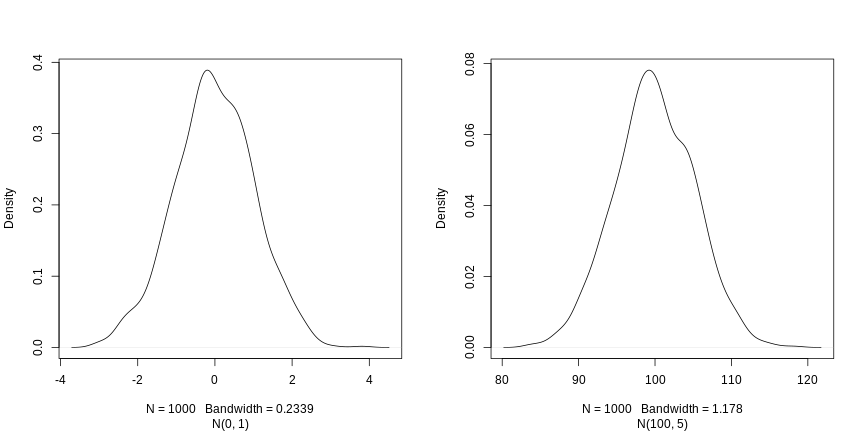
The three arguments, n, mean and
sd, define the size of the sample, and the parameters of
the normal distribution, i.e the mean and its standard deviation. The
defaults of the latter are 0 and 1.
R
rnorm(5)
OUTPUT
[1] 0.69641761 0.05351568 -1.31028350 -2.12306606 -0.20807859R
rnorm(5, 2, 2)
OUTPUT
[1] 1.3744268 -0.1164714 2.8344472 1.3690969 3.6510983R
rnorm(5, 100, 5)
OUTPUT
[1] 106.45636 96.87448 95.62427 100.71678 107.12595Now that we have learned how to write scripts, and the basics of R’s data structures, we are ready to start working with larger data, and learn about data frames.
- How to interact with R