Next steps
Last updated on 2026-07-14 | Edit this page
Overview
Questions
- What is a
SummarizedExperiment? - What is Bioconductor?
Objectives
- Introduce the Bioconductor project.
- Introduce the notion of data containers.
- Give an overview of the
SummarizedExperiment, extensively used in omics analyses.
Next steps
Data in bioinformatics is often complex. To deal with this, developers define specialised data containers (termed classes) that match the properties of the data they need to handle.
This aspect is central to the Bioconductor1 project which uses the same core data infrastructure across packages. This certainly contributed to Bioconductor’s success. Bioconductor package developers are advised to make use of existing infrastructure to provide coherence, interoperability, and stability to the project as a whole.
To illustrate such an omics data container, we’ll present the
SummarizedExperiment class.
SummarizedExperiment
The figure below represents the anatomy of the SummarizedExperiment class.

Objects of the class SummarizedExperiment contain :
One (or more) assay(s) containing the quantitative omics data (expression data), stored as a matrix-like object. Features (genes, transcripts, proteins, …) are defined along the rows, and samples along the columns.
A sample metadata slot containing sample co-variates, stored as a data frame. Rows from this table represent samples (rows match exactly the columns of the expression data).
A feature metadata slot containing feature co-variates, stored as a data frame. The rows of this data frame match exactly the rows of the expression data.
The coordinated nature of the SummarizedExperiment
guarantees that during data manipulation, the dimensions of the
different slots will always match (i.e the columns in the expression
data and then rows in the sample metadata, as well as the rows in the
expression data and feature metadata) during data manipulation. For
example, if we had to exclude one sample from the assay, it would be
automatically removed from the sample metadata in the same
operation.
The metadata slots can grow additional co-variates (columns) without affecting the other structures.
Creating a SummarizedExperiment
In order to create a SummarizedExperiment, we will
create the individual components, i.e the count matrix, the sample and
gene metadata from csv files. These are typically how RNA-Seq data are
provided (after raw data have been processed).
-
An expression matrix: we load the count matrix,
specifying that the first columns contains row/gene names, and convert
the
data.frameto amatrix. You can download it by clicking this link.
R
count_matrix <- read.csv("data/count_matrix.csv",
                         row.names = 1) |>
    as.matrix()

count_matrix[1:5, ]
OUTPUT
        GSM2545336 GSM2545337 GSM2545338 GSM2545339 GSM2545340 GSM2545341
Asl           1170        361        400        586        626        988
Apod         36194      10347       9173      10620      13021      29594
Cyp2d22       4060       1616       1603       1901       2171       3349
Klk6           287        629        641        578        448        195
Fcrls           85        233        244        237        180         38
        GSM2545342 GSM2545343 GSM2545344 GSM2545345 GSM2545346 GSM2545347
Asl            836        535        586        597        938       1035
Apod         24959      13668      13230      15868      27769      34301
Cyp2d22       3122       2008       2254       2277       2985       3452
Klk6           186       1101        537        567        327        233
Fcrls           68        375        199        177         89         67
        GSM2545348 GSM2545349 GSM2545350 GSM2545351 GSM2545352 GSM2545353
Asl            494        481        666        937        803        541
Apod         11258      11812      15816      29242      20415      13682
Cyp2d22       1883       2014       2417       3678       2920       2216
Klk6           742        881        828        250        798        710
Fcrls          300        233        231         81        303        285
        GSM2545354 GSM2545362 GSM2545363 GSM2545380
Asl            473        748        576       1192
Apod         11088      15916      11166      38148
Cyp2d22       1821       2842       2011       4019
Klk6           894        501        598        259
Fcrls          248        179        184         68
R
dim(count_matrix)
OUTPUT
[1] 1474 22- A table describing the samples, available at this link.
R
sample_metadata <- read.csv("data/sample_metadata.csv")
sample_metadata
OUTPUT
       sample     organism age    sex   infection  strain time     tissue mouse
1  GSM2545336 Mus musculus   8 Female  InfluenzaA C57BL/6    8 Cerebellum    14
2  GSM2545337 Mus musculus   8 Female NonInfected C57BL/6    0 Cerebellum     9
3  GSM2545338 Mus musculus   8 Female NonInfected C57BL/6    0 Cerebellum    10
4  GSM2545339 Mus musculus   8 Female  InfluenzaA C57BL/6    4 Cerebellum    15
5  GSM2545340 Mus musculus   8   Male  InfluenzaA C57BL/6    4 Cerebellum    18
6  GSM2545341 Mus musculus   8   Male  InfluenzaA C57BL/6    8 Cerebellum     6
7  GSM2545342 Mus musculus   8 Female  InfluenzaA C57BL/6    8 Cerebellum     5
8  GSM2545343 Mus musculus   8   Male NonInfected C57BL/6    0 Cerebellum    11
9  GSM2545344 Mus musculus   8 Female  InfluenzaA C57BL/6    4 Cerebellum    22
10 GSM2545345 Mus musculus   8   Male  InfluenzaA C57BL/6    4 Cerebellum    13
11 GSM2545346 Mus musculus   8   Male  InfluenzaA C57BL/6    8 Cerebellum    23
12 GSM2545347 Mus musculus   8   Male  InfluenzaA C57BL/6    8 Cerebellum    24
13 GSM2545348 Mus musculus   8 Female NonInfected C57BL/6    0 Cerebellum     8
14 GSM2545349 Mus musculus   8   Male NonInfected C57BL/6    0 Cerebellum     7
15 GSM2545350 Mus musculus   8   Male  InfluenzaA C57BL/6    4 Cerebellum     1
16 GSM2545351 Mus musculus   8 Female  InfluenzaA C57BL/6    8 Cerebellum    16
17 GSM2545352 Mus musculus   8 Female  InfluenzaA C57BL/6    4 Cerebellum    21
18 GSM2545353 Mus musculus   8 Female NonInfected C57BL/6    0 Cerebellum     4
19 GSM2545354 Mus musculus   8   Male NonInfected C57BL/6    0 Cerebellum     2
20 GSM2545362 Mus musculus   8 Female  InfluenzaA C57BL/6    4 Cerebellum    20
21 GSM2545363 Mus musculus   8   Male  InfluenzaA C57BL/6    4 Cerebellum    12
22 GSM2545380 Mus musculus   8 Female  InfluenzaA C57BL/6    8 Cerebellum    19
R
dim(sample_metadata)
OUTPUT
[1] 22 9- A table describing the genes, available at this link.
R
gene_metadata <- read.csv("data/gene_metadata.csv")
gene_metadata[1:10, 1:4]
OUTPUT
      gene ENTREZID
1      Asl   109900
2     Apod    11815
3  Cyp2d22    56448
4     Klk6    19144
5    Fcrls    80891
6   Slc2a4    20528
7     Exd2    97827
8     Gjc2   118454
9     Plp1    18823
10    Gnb4    14696
                                                                         product
1                                 argininosuccinate lyase, transcript variant X1
2                                         apolipoprotein D, transcript variant 3
3   cytochrome P450, family 2, subfamily d, polypeptide 22, transcript variant 2
4                           kallikrein related-peptidase 6, transcript variant 2
5                  Fc receptor-like S, scavenger receptor, transcript variant X1
6            solute carrier family 2 (facilitated glucose transporter), member 4
7                                          exonuclease 3'-5' domain containing 2
8                            gap junction protein, gamma 2, transcript variant 1
9                           proteolipid protein (myelin) 1, transcript variant 1
10 guanine nucleotide binding protein (G protein), beta 4, transcript variant X2
      ensembl_gene_id
1  ENSMUSG00000025533
2  ENSMUSG00000022548
3  ENSMUSG00000061740
4  ENSMUSG00000050063
5  ENSMUSG00000015852
6  ENSMUSG00000018566
7  ENSMUSG00000032705
8  ENSMUSG00000043448
9  ENSMUSG00000031425
10 ENSMUSG00000027669
R
dim(gene_metadata)
OUTPUT
[1] 1474 9We will create a SummarizedExperiment from these
tables:
The count matrix that will be used as the
assayThe table describing the samples will be used as the sample metadata slot
The table describing the genes will be used as the features metadata slot
To do this we can put the different parts together using the
SummarizedExperiment constructor:
R
## BiocManager::install("SummarizedExperiment")
library("SummarizedExperiment")
First, we make sure that the samples are in the same order in the count matrix and the sample annotation, and the same for the genes in the count matrix and the gene annotation.
R
stopifnot(rownames(count_matrix) == gene_metadata$gene)
stopifnot(colnames(count_matrix) == sample_metadata$sample)
R
se <- SummarizedExperiment(assays = list(counts = count_matrix),
                           colData = sample_metadata,
                           rowData = gene_metadata)
se
OUTPUT
class: SummarizedExperiment
dim: 1474 22
metadata(0):
assays(1): counts
rownames(1474): Asl Apod ... Lmx1a Pbx1
rowData names(9): gene ENTREZID ... phenotype_description
  hsapiens_homolog_associated_gene_name
colnames(22): GSM2545336 GSM2545337 ... GSM2545363 GSM2545380
colData names(9): sample organism ... tissue mouse
Saving data
Exporting data to a spreadsheet, as we did in a previous episode, has
several limitations, such as those described in the first chapter
(possible inconsistencies with , and . for
decimal separators and lack of variable type definitions). Furthermore,
exporting data to a spreadsheet is only relevant for rectangular data
such as dataframes and matrices.
A more general way to save data, that is specific to R and is
guaranteed to work on any operating system, is to use the
saveRDS function. Saving objects like this will generate a
binary representation on disk (using the rds file extension
here), which can be loaded back into R using the readRDS
function.
R
saveRDS(se, file = "data_output/se.rds")
rm(se)
se <- readRDS("data_output/se.rds")
head(se)
To conclude, when it comes to saving data from R that will be loaded
again in R, saving and loading with saveRDS and
readRDS is the preferred approach. If tabular data need to
be shared with somebody that is not using R, then exporting to a
text-based spreadsheet is a good alternative.
Using this data structure, we can access the expression matrix with
the assay function:
R
head(assay(se))
OUTPUT
        GSM2545336 GSM2545337 GSM2545338 GSM2545339 GSM2545340 GSM2545341
Asl           1170        361        400        586        626        988
Apod         36194      10347       9173      10620      13021      29594
Cyp2d22       4060       1616       1603       1901       2171       3349
Klk6           287        629        641        578        448        195
Fcrls           85        233        244        237        180         38
Slc2a4         782        231        248        265        313        786
        GSM2545342 GSM2545343 GSM2545344 GSM2545345 GSM2545346 GSM2545347
Asl            836        535        586        597        938       1035
Apod         24959      13668      13230      15868      27769      34301
Cyp2d22       3122       2008       2254       2277       2985       3452
Klk6           186       1101        537        567        327        233
Fcrls           68        375        199        177         89         67
Slc2a4         528        249        266        357        654        693
        GSM2545348 GSM2545349 GSM2545350 GSM2545351 GSM2545352 GSM2545353
Asl            494        481        666        937        803        541
Apod         11258      11812      15816      29242      20415      13682
Cyp2d22       1883       2014       2417       3678       2920       2216
Klk6           742        881        828        250        798        710
Fcrls          300        233        231         81        303        285
Slc2a4         271        304        349        715        513        320
        GSM2545354 GSM2545362 GSM2545363 GSM2545380
Asl            473        748        576       1192
Apod         11088      15916      11166      38148
Cyp2d22       1821       2842       2011       4019
Klk6           894        501        598        259
Fcrls          248        179        184         68
Slc2a4         248        350        317        796
R
dim(assay(se))
OUTPUT
[1] 1474 22We can access the sample metadata using the colData
function:
R
colData(se)
OUTPUT
DataFrame with 22 rows and 9 columns
                sample     organism       age         sex   infection
           <character>  <character> <integer> <character> <character>
GSM2545336  GSM2545336 Mus musculus         8      Female  InfluenzaA
GSM2545337  GSM2545337 Mus musculus         8      Female NonInfected
GSM2545338  GSM2545338 Mus musculus         8      Female NonInfected
GSM2545339  GSM2545339 Mus musculus         8      Female  InfluenzaA
GSM2545340  GSM2545340 Mus musculus         8        Male  InfluenzaA
...                ...          ...       ...         ...         ...
GSM2545353  GSM2545353 Mus musculus         8      Female NonInfected
GSM2545354  GSM2545354 Mus musculus         8        Male NonInfected
GSM2545362  GSM2545362 Mus musculus         8      Female  InfluenzaA
GSM2545363  GSM2545363 Mus musculus         8        Male  InfluenzaA
GSM2545380  GSM2545380 Mus musculus         8      Female  InfluenzaA
                strain      time      tissue     mouse
           <character> <integer> <character> <integer>
GSM2545336     C57BL/6         8  Cerebellum        14
GSM2545337     C57BL/6         0  Cerebellum         9
GSM2545338     C57BL/6         0  Cerebellum        10
GSM2545339     C57BL/6         4  Cerebellum        15
GSM2545340     C57BL/6         4  Cerebellum        18
...                ...       ...         ...       ...
GSM2545353     C57BL/6         0  Cerebellum         4
GSM2545354     C57BL/6         0  Cerebellum         2
GSM2545362     C57BL/6         4  Cerebellum        20
GSM2545363     C57BL/6         4  Cerebellum        12
GSM2545380     C57BL/6         8  Cerebellum        19
R
dim(colData(se))
OUTPUT
[1] 22 9We can also access the feature metadata using the
rowData function:
R
head(rowData(se))
OUTPUT
DataFrame with 6 rows and 9 columns
               gene  ENTREZID                product    ensembl_gene_id
        <character> <integer>            <character>        <character>
Asl             Asl    109900 argininosuccinate ly.. ENSMUSG00000025533
Apod           Apod     11815 apolipoprotein D, tr.. ENSMUSG00000022548
Cyp2d22     Cyp2d22     56448 cytochrome P450, fam.. ENSMUSG00000061740
Klk6           Klk6     19144 kallikrein related-p.. ENSMUSG00000050063
Fcrls         Fcrls     80891 Fc receptor-like S, .. ENSMUSG00000015852
Slc2a4       Slc2a4     20528 solute carrier famil.. ENSMUSG00000018566
        external_synonym chromosome_name   gene_biotype  phenotype_description
             <character>     <character>    <character>            <character>
Asl        2510006M18Rik               5 protein_coding abnormal circulating..
Apod                  NA              16 protein_coding abnormal lipid homeo..
Cyp2d22             2D22              15 protein_coding abnormal skin morpho..
Klk6                Bssp               7 protein_coding abnormal cytokine le..
Fcrls      2810439C17Rik               3 protein_coding decreased CD8-positi..
Slc2a4            Glut-4              11 protein_coding abnormal circulating..
        hsapiens_homolog_associated_gene_name
                                  <character>
Asl                                       ASL
Apod                                     APOD
Cyp2d22                                CYP2D6
Klk6                                     KLK6
Fcrls                                   FCRL2
Slc2a4                                 SLC2A4
R
dim(rowData(se))
OUTPUT
[1] 1474 9Subsetting a SummarizedExperiment
SummarizedExperiment can be subset just like with data frames, with numerics or with characters of logicals.
Below, we create a new instance of class SummarizedExperiment that contains only the 5 first features for the 3 first samples.
R
se1 <- se[1:5, 1:3]
se1
OUTPUT
class: SummarizedExperiment
dim: 5 3
metadata(0):
assays(1): counts
rownames(5): Asl Apod Cyp2d22 Klk6 Fcrls
rowData names(9): gene ENTREZID ... phenotype_description
  hsapiens_homolog_associated_gene_name
colnames(3): GSM2545336 GSM2545337 GSM2545338
colData names(9): sample organism ... tissue mouse
R
colData(se1)
OUTPUT
DataFrame with 3 rows and 9 columns
                sample     organism       age         sex   infection
           <character>  <character> <integer> <character> <character>
GSM2545336  GSM2545336 Mus musculus         8      Female  InfluenzaA
GSM2545337  GSM2545337 Mus musculus         8      Female NonInfected
GSM2545338  GSM2545338 Mus musculus         8      Female NonInfected
                strain      time      tissue     mouse
           <character> <integer> <character> <integer>
GSM2545336     C57BL/6         8  Cerebellum        14
GSM2545337     C57BL/6         0  Cerebellum         9
GSM2545338     C57BL/6         0  Cerebellum        10
R
rowData(se1)
OUTPUT
DataFrame with 5 rows and 9 columns
               gene  ENTREZID                product    ensembl_gene_id
        <character> <integer>            <character>        <character>
Asl             Asl    109900 argininosuccinate ly.. ENSMUSG00000025533
Apod           Apod     11815 apolipoprotein D, tr.. ENSMUSG00000022548
Cyp2d22     Cyp2d22     56448 cytochrome P450, fam.. ENSMUSG00000061740
Klk6           Klk6     19144 kallikrein related-p.. ENSMUSG00000050063
Fcrls         Fcrls     80891 Fc receptor-like S, .. ENSMUSG00000015852
        external_synonym chromosome_name   gene_biotype  phenotype_description
             <character>     <character>    <character>            <character>
Asl        2510006M18Rik               5 protein_coding abnormal circulating..
Apod                  NA              16 protein_coding abnormal lipid homeo..
Cyp2d22             2D22              15 protein_coding abnormal skin morpho..
Klk6                Bssp               7 protein_coding abnormal cytokine le..
Fcrls      2810439C17Rik               3 protein_coding decreased CD8-positi..
        hsapiens_homolog_associated_gene_name
                                  <character>
Asl                                       ASL
Apod                                     APOD
Cyp2d22                                CYP2D6
Klk6                                     KLK6
Fcrls                                   FCRL2
We can also use the colData() function to subset on
something from the sample metadata or the rowData() to
subset on something from the feature metadata. For example, here we keep
only miRNAs and the non infected samples:
R
se1 <- se[rowData(se)$gene_biotype == "miRNA",
          colData(se)$infection == "NonInfected"]
se1
OUTPUT
class: SummarizedExperiment
dim: 7 7
metadata(0):
assays(1): counts
rownames(7): Mir1901 Mir378a ... Mir128-1 Mir7682
rowData names(9): gene ENTREZID ... phenotype_description
  hsapiens_homolog_associated_gene_name
colnames(7): GSM2545337 GSM2545338 ... GSM2545353 GSM2545354
colData names(9): sample organism ... tissue mouse
R
assay(se1)
OUTPUT
         GSM2545337 GSM2545338 GSM2545343 GSM2545348 GSM2545349 GSM2545353
Mir1901          45         44         74         55         68         33
Mir378a          11          7          9          4         12          4
Mir133b           4          6          5          4          6          7
Mir30c-2         10          6         16         12          8         17
Mir149            1          2          0          0          0          0
Mir128-1          4          1          2          2          1          2
Mir7682           2          0          4          1          3          5
         GSM2545354
Mir1901          60
Mir378a           8
Mir133b           3
Mir30c-2         15
Mir149            2
Mir128-1          1
Mir7682           5
R
colData(se1)
OUTPUT
DataFrame with 7 rows and 9 columns
                sample     organism       age         sex   infection
           <character>  <character> <integer> <character> <character>
GSM2545337  GSM2545337 Mus musculus         8      Female NonInfected
GSM2545338  GSM2545338 Mus musculus         8      Female NonInfected
GSM2545343  GSM2545343 Mus musculus         8        Male NonInfected
GSM2545348  GSM2545348 Mus musculus         8      Female NonInfected
GSM2545349  GSM2545349 Mus musculus         8        Male NonInfected
GSM2545353  GSM2545353 Mus musculus         8      Female NonInfected
GSM2545354  GSM2545354 Mus musculus         8        Male NonInfected
                strain      time      tissue     mouse
           <character> <integer> <character> <integer>
GSM2545337     C57BL/6         0  Cerebellum         9
GSM2545338     C57BL/6         0  Cerebellum        10
GSM2545343     C57BL/6         0  Cerebellum        11
GSM2545348     C57BL/6         0  Cerebellum         8
GSM2545349     C57BL/6         0  Cerebellum         7
GSM2545353     C57BL/6         0  Cerebellum         4
GSM2545354     C57BL/6         0  Cerebellum         2
R
rowData(se1)
OUTPUT
DataFrame with 7 rows and 9 columns
                gene  ENTREZID        product    ensembl_gene_id
         <character> <integer>    <character>        <character>
Mir1901      Mir1901 100316686  microRNA 1901 ENSMUSG00000084565
Mir378a      Mir378a    723889  microRNA 378a ENSMUSG00000105200
Mir133b      Mir133b    723817  microRNA 133b ENSMUSG00000065480
Mir30c-2    Mir30c-2    723964 microRNA 30c-2 ENSMUSG00000065567
Mir149        Mir149    387167   microRNA 149 ENSMUSG00000065470
Mir128-1    Mir128-1    387147 microRNA 128-1 ENSMUSG00000065520
Mir7682      Mir7682 102466847  microRNA 7682 ENSMUSG00000106406
         external_synonym chromosome_name gene_biotype  phenotype_description
              <character>     <character>  <character>            <character>
Mir1901          Mirn1901              18        miRNA                     NA
Mir378a           Mirn378              18        miRNA abnormal mitochondri..
Mir133b          mir 133b               1        miRNA no abnormal phenotyp..
Mir30c-2        mir 30c-2               1        miRNA                     NA
Mir149            Mirn149               1        miRNA increased circulatin..
Mir128-1          Mirn128               1        miRNA no abnormal phenotyp..
Mir7682      mmu-mir-7682               1        miRNA                     NA
         hsapiens_homolog_associated_gene_name
                                   <character>
Mir1901                                     NA
Mir378a                                MIR378A
Mir133b                                MIR133B
Mir30c-2                               MIR30C2
Mir149                                      NA
Mir128-1                              MIR128-1
Mir7682                                     NA
Challenge
Extract the gene expression levels of the 3 first genes in samples at time 0 and at time 8.
R
assay(se)[1:3, colData(se)$time != 4]
OUTPUT
        GSM2545336 GSM2545337 GSM2545338 GSM2545341 GSM2545342 GSM2545343
Asl           1170        361        400        988        836        535
Apod         36194      10347       9173      29594      24959      13668
Cyp2d22       4060       1616       1603       3349       3122       2008
        GSM2545346 GSM2545347 GSM2545348 GSM2545349 GSM2545351 GSM2545353
Asl            938       1035        494        481        937        541
Apod         27769      34301      11258      11812      29242      13682
Cyp2d22       2985       3452       1883       2014       3678       2216
        GSM2545354 GSM2545380
Asl            473       1192
Apod         11088      38148
Cyp2d22       1821       4019
R
# Equivalent to
assay(se)[1:3, colData(se)$time == 0 | colData(se)$time == 8]
OUTPUT
        GSM2545336 GSM2545337 GSM2545338 GSM2545341 GSM2545342 GSM2545343
Asl           1170        361        400        988        836        535
Apod         36194      10347       9173      29594      24959      13668
Cyp2d22       4060       1616       1603       3349       3122       2008
        GSM2545346 GSM2545347 GSM2545348 GSM2545349 GSM2545351 GSM2545353
Asl            938       1035        494        481        937        541
Apod         27769      34301      11258      11812      29242      13682
Cyp2d22       2985       3452       1883       2014       3678       2216
        GSM2545354 GSM2545380
Asl            473       1192
Apod         11088      38148
Cyp2d22       1821       4019
Challenge
Verify that you get the same values using the long rna
table.
R
rna |>
    filter(gene %in% c("Asl", "Apod", "Cyd2d22")) |>
    filter(time != 4) |>
    select(expression)
OUTPUT
# A tibble: 28 × 1
   expression
        <dbl>
 1       1170
 2      36194
 3        361
 4      10347
 5        400
 6       9173
 7        988
 8      29594
 9        836
10      24959
# ℹ 18 more rows
The long table and the SummarizedExperiment contain the
same information, but are simply structured differently. Each approach
has its own advantages: the former is a good fit for the
tidyverse packages, while the latter is the preferred
structure for many bioinformatics and statistical processing steps. For
example, a typical RNA-Seq analyses using the DESeq2
package.
Adding variables to metadata
We can also add information to the metadata. Suppose that you want to add the center where the samples were collected…
R
colData(se)$center <- rep("University of Illinois", nrow(colData(se)))
colData(se)
OUTPUT
DataFrame with 22 rows and 10 columns
                sample     organism       age         sex   infection
           <character>  <character> <integer> <character> <character>
GSM2545336  GSM2545336 Mus musculus         8      Female  InfluenzaA
GSM2545337  GSM2545337 Mus musculus         8      Female NonInfected
GSM2545338  GSM2545338 Mus musculus         8      Female NonInfected
GSM2545339  GSM2545339 Mus musculus         8      Female  InfluenzaA
GSM2545340  GSM2545340 Mus musculus         8        Male  InfluenzaA
...                ...          ...       ...         ...         ...
GSM2545353  GSM2545353 Mus musculus         8      Female NonInfected
GSM2545354  GSM2545354 Mus musculus         8        Male NonInfected
GSM2545362  GSM2545362 Mus musculus         8      Female  InfluenzaA
GSM2545363  GSM2545363 Mus musculus         8        Male  InfluenzaA
GSM2545380  GSM2545380 Mus musculus         8      Female  InfluenzaA
                strain      time      tissue     mouse                 center
           <character> <integer> <character> <integer>            <character>
GSM2545336     C57BL/6         8  Cerebellum        14 University of Illinois
GSM2545337     C57BL/6         0  Cerebellum         9 University of Illinois
GSM2545338     C57BL/6         0  Cerebellum        10 University of Illinois
GSM2545339     C57BL/6         4  Cerebellum        15 University of Illinois
GSM2545340     C57BL/6         4  Cerebellum        18 University of Illinois
...                ...       ...         ...       ...                    ...
GSM2545353     C57BL/6         0  Cerebellum         4 University of Illinois
GSM2545354     C57BL/6         0  Cerebellum         2 University of Illinois
GSM2545362     C57BL/6         4  Cerebellum        20 University of Illinois
GSM2545363     C57BL/6         4  Cerebellum        12 University of Illinois
GSM2545380     C57BL/6         8  Cerebellum        19 University of Illinois
This illustrates that the metadata slots can grow indefinitely without affecting the other structures!
tidySummarizedExperiment
You may be wondering, can we use tidyverse commands to interact with
SummarizedExperiment objects? The answer is yes, we can
with the tidySummarizedExperiment package.
Remember what our SummarizedExperiment object looks like:
R
se
OUTPUT
class: SummarizedExperiment
dim: 1474 22
metadata(0):
assays(1): counts
rownames(1474): Asl Apod ... Lmx1a Pbx1
rowData names(9): gene ENTREZID ... phenotype_description
  hsapiens_homolog_associated_gene_name
colnames(22): GSM2545336 GSM2545337 ... GSM2545363 GSM2545380
colData names(10): sample organism ... mouse center
Load tidySummarizedExperiment and then take a look at
the se object again.
R
#BiocManager::install("tidySummarizedExperiment")
library("tidySummarizedExperiment")

se
OUTPUT
class: SummarizedExperiment
dim: 1474 22
metadata(0):
assays(1): counts
rownames(1474): Asl Apod ... Lmx1a Pbx1
rowData names(9): gene ENTREZID ... phenotype_description
  hsapiens_homolog_associated_gene_name
colnames(22): GSM2545336 GSM2545337 ... GSM2545363 GSM2545380
colData names(10): sample organism ... mouse center
It’s still a SummarizedExperiment object, so maintains
the efficient structure, but now we can view it as a tibble. Note the
first line of the output says this, it’s a
SummarizedExperiment-tibble abstraction. We
can also see in the second line of the output the number of transcripts
and samples.
If we want to revert to the standard
SummarizedExperiment view, we can do that.
R
options("restore_SummarizedExperiment_show" = TRUE)
se
OUTPUT
class: SummarizedExperiment
dim: 1474 22
metadata(0):
assays(1): counts
rownames(1474): Asl Apod ... Lmx1a Pbx1
rowData names(9): gene ENTREZID ... phenotype_description
  hsapiens_homolog_associated_gene_name
colnames(22): GSM2545336 GSM2545337 ... GSM2545363 GSM2545380
colData names(10): sample organism ... mouse center
But here we use the tibble view.
R
options("restore_SummarizedExperiment_show" = FALSE)
se
OUTPUT
class: SummarizedExperiment
dim: 1474 22
metadata(0):
assays(1): counts
rownames(1474): Asl Apod ... Lmx1a Pbx1
rowData names(9): gene ENTREZID ... phenotype_description
  hsapiens_homolog_associated_gene_name
colnames(22): GSM2545336 GSM2545337 ... GSM2545363 GSM2545380
colData names(10): sample organism ... mouse center
We can now use tidyverse commands to interact with the
SummarizedExperiment object.
We can use filter to filter for rows using a condition
e.g. to view all rows for one sample.
R
se |> filter(.sample == "GSM2545336")
ERROR
Error in `dplyr_fn()` at tidySummarizedExperiment/R/query_scope_analysis.R:481:3:
ℹ In argument: `.sample == "GSM2545336"`.
Caused by error:
! object '.sample' not found
We can use select to specify columns we want to
view.
R
se |> select(.sample)
WARNING
Warning: `when()` was deprecated in purrr 1.0.0.
ℹ Please use `if` instead.
ℹ The deprecated feature was likely used in the tidySummarizedExperiment
  package.
  Please report the issue at
  <https://github.com/stemangiola/tidySummarizedExperiment/issues>.
This warning is displayed once per session.
Call `lifecycle::last_lifecycle_warnings()` to see where this warning was
generated.
OUTPUT
tidySummarizedExperiment says: Key columns are missing. A data frame is returned for independent data analysis.OUTPUT
# A tibble: 32,428 × 1
   .sample
   <chr>
 1 GSM2545336
 2 GSM2545336
 3 GSM2545336
 4 GSM2545336
 5 GSM2545336
 6 GSM2545336
 7 GSM2545336
 8 GSM2545336
 9 GSM2545336
10 GSM2545336
# ℹ 32,418 more rows
We can use mutate to add metadata info.
R
se |> mutate(center = "Heidelberg University")
OUTPUT
class: SummarizedExperiment
dim: 1474 22
metadata(1): latest_mutate_scope_report
assays(1): counts
rownames(1474): Asl Apod ... Lmx1a Pbx1
rowData names(9): gene ENTREZID ... phenotype_description
  hsapiens_homolog_associated_gene_name
colnames(22): GSM2545336 GSM2545337 ... GSM2545363 GSM2545380
colData names(10): sample organism ... mouse center
We can also combine commands with the tidyverse pipe
|>. For example, we could combine group_by
and summarise to get the total counts for each sample.
R
se |>
    group_by(.sample) |>
    summarise(total_counts=sum(counts))
OUTPUT
tidySummarizedExperiment says: A data frame is returned for independent data analysis.OUTPUT
# A tibble: 22 × 2
.sample total_counts
<chr> <int>
1 GSM2545336 3039671
2 GSM2545337 2602360
3 GSM2545338 2458618
4 GSM2545339 2500082
5 GSM2545340 2479024
6 GSM2545341 2413723
7 GSM2545342 2349728
8 GSM2545343 3105652
9 GSM2545344 2524137
10 GSM2545345 2506038
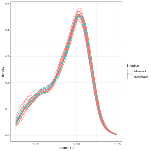
# ℹ 12 more rowsWe can treat the tidy SummarizedExperiment object as a normal tibble for plotting.
Here we plot the distribution of counts per sample.
R
se |>
    ggplot(aes(counts + 1, group=.sample, color=infection)) +
    geom_density() +
    scale_x_log10() +
    theme_bw()
For more information on tidySummarizedExperiment, see
the package
website.
Take-home message
SummarizedExperimentrepresents an efficient way to store and handle omics data.They are used in many Bioconductor packages.
If you follow the next training focused on RNA sequencing analysis,
you will learn to use the Bioconductor DESeq2 package to do
some differential expression analyses. The whole analysis of the
DESeq2 package is handled in a
SummarizedExperiment.
- Bioconductor is a project provide support and packages for the comprehension of high high-throughput biology data.
- A
SummarizedExperimentis a type of object useful to store and manage high-throughput omics data.
The Bioconductor was initiated by Robert Gentleman, one of the two creators of the R language. Bioconductor provides tools dedicated to omics data analysis. Bioconductor uses the R statistical programming language and is open source and open development.↩︎