Power Calculations

Overview

Teaching: 0 min
Exercises: 0 min

Questions

• What is statistical power?

• How is power calculated?

Objectives

Power Calculations

Introduction

We have used the example of the effects of two different diets on the weight of mice. Since in this illustrative example we have access to the population, we know that in fact there is a substantial (about 10%) difference between the average weights of the two populations:

library(dplyr)
pheno <- read.csv("../data/mice_pheno.csv") #Previously downloaded 

controlPopulation <- filter(pheno, Sex == "F" & Diet == "chow") %>%  
  select(Bodyweight) %>% unlist

hfPopulation <- filter(pheno, Sex == "F" & Diet == "hf") %>%  
  select(Bodyweight) %>% unlist

mu_hf <- mean(hfPopulation)
mu_control <- mean(controlPopulation)
print(mu_hf - mu_control)

[1] 2.375517

print((mu_hf - mu_control)/mu_control * 100) #percent increase

[1] 9.942157

We have also seen that, in some cases, when we take a sample and perform a t-test, we don’t always get a p-value smaller than 0.05. For example, here is a case where we take a sample of 5 mice and don’t achieve statistical significance at the 0.05 level:

set.seed(1)
N <- 5
hf <- sample(hfPopulation, N)
control <- sample(controlPopulation, N)
t.test(hf, control)$p.value

[1] 0.5806661

Did we make a mistake? By not rejecting the null hypothesis, are we saying the diet has no effect? The answer to this question is no. All we can say is that we did not reject the null hypothesis. But this does not necessarily imply that the null is true. The problem is that, in this particular instance, we don’t have enough power, a term we are now going to define. If you are doing scientific research, it is very likely that you will have to do a power calculation at some point. In many cases, it is an ethical obligation as it can help you avoid sacrificing mice unnecessarily or limiting the number of human subjects exposed to potential risk in a study. Here we explain what statistical power means.

Types of Error

Whenever we perform a statistical test, we are aware that we may make a mistake. This is why our p-values are not 0. Under the null, there is always a positive, perhaps very small, but still positive chance that we will reject the null when it is true. If the p-value is 0.05, it will happen 1 out of 20 times. This error is called type I error by statisticians.

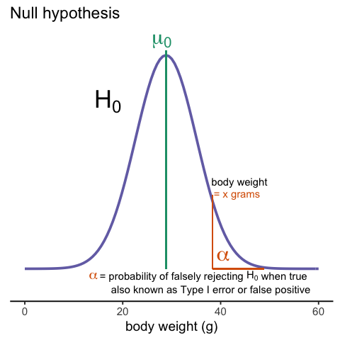
A type I error is defined as rejecting the null when we should not. This is also referred to as a false positive. So why do we then use 0.05? Shouldn’t we use 0.000001 to be really sure? The reason we don’t use infinitesimal cut-offs to avoid type I errors at all cost is that there is another error we can commit: to not reject the null when we should. This is called a type II error or a false negative.

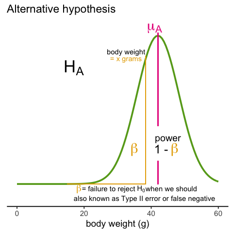
The R code analysis above shows an example of a false negative: we did not reject the null hypothesis (at the 0.05 level) and, because we happen to know and peeked at the true population means, we know there is in fact a difference. Had we used a p-value cutoff of 0.25, we would not have made this mistake. However, in general, are we comfortable with a type I error rate of 1 in 4? Usually we are not.

The 0.05 and 0.01 Cut-offs Are Arbitrary

Most journals and regulatory agencies frequently insist that results be significant at the 0.01 or 0.05 levels. Of course there is nothing special about these numbers other than the fact that some of the first papers on p-values used these values as examples. Part of the goal of this book is to give readers a good understanding of what p-values and confidence intervals are so that these choices can be judged in an informed way. Unfortunately, in science, these cut-offs are applied somewhat mindlessly, but that topic is part of a complicated debate.

Power Calculation

Power is the probability of rejecting the null when the null is false. Of course “when the null is false” is a complicated statement because it can be false in many ways.

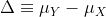
could be anything and the power actually depends on this parameter. It also depends on the standard error of your estimates which in turn depends on the sample size and the population standard deviations. In practice, we don’t know these so we usually report power for several plausible values of Δ, σ_X, σ_Y and various sample sizes. Statistical theory gives us formulas to calculate power. The pwr package performs these calculations for you. Here we will illustrate the concepts behind power by coding up simulations in R.

Suppose our sample size is:

N <- 12

and we will reject the null hypothesis at:

alpha <- 0.05

What is our power with this particular data? We will compute this probability by re-running the exercise many times and calculating the proportion of times the null hypothesis is rejected. Specifically, we will run:

B <- 2000

simulations. The simulation is as follows: we take a sample of size N from both control and treatment groups, we perform a t-test comparing these two, and report if the p-value is less than alpha or not. We write a function that does this:

reject <- function(N, alpha=0.05){
   hf <- sample(hfPopulation, N) 
   control <- sample(controlPopulation, N)
   pval <- t.test(hf, control)$p.value
   pval < alpha
}

Here is an example of one simulation for a sample size of 12. The call to reject answers the question “Did we reject?”

reject(12)

[1] TRUE

Now we can use the replicate function to do this B times.

rejections <- replicate(B, reject(N))

Our power is just the proportion of times we correctly reject. So with N = 12 our power is only:

mean(rejections)

[1] 0.2155

This explains why the t-test was not rejecting when we knew the null was false. With a sample size of just 12, our power is about 23%. To guard against false positives at the 0.05 level, we had set the threshold at a high enough level that resulted in many type II errors.

Let’s see how power improves with N. We will use the function sapply, which applies a function to each of the elements of a vector. We want to repeat the above for the following sample size:

Ns <- seq(5, 50, 5)

So we use apply like this:

power <- sapply(Ns,function(N){
  rejections <- replicate(B, reject(N))
  mean(rejections)
  })

For each of the three simulations, the above code returns the proportion of times we reject. Not surprisingly power increases with N:

plot(Ns, power, type="b")

Similarly, if we change the level alpha at which we reject, power changes. The smaller I want the chance of type I error to be, the less power I will have. Another way of saying this is that we trade off between the two types of error. We can see this by writing similar code, but keeping N fixed and considering several values of alpha:

N <- 30
alphas <- c(0.1, 0.05, 0.01, 0.001, 0.0001)
power <- sapply(alphas, function(alpha){
  rejections <- replicate(B, reject(N, alpha=alpha))
  mean(rejections)
})
plot(alphas, power, xlab="alpha", type="b", log="x")

Note that the x-axis in this last plot is in the log scale.

There is no “right” power or “right” alpha level, but it is important that you understand what each means.

To see this clearly, you could create a plot with curves of power versus N. Show several curves in the same plot with color representing alpha level.

p-values Are Arbitrary under the Alternative Hypothesis

Another consequence of what we have learned about power is that p-values are somewhat arbitrary when the null hypothesis is not true and therefore the alternative hypothesis is true (the difference between the population means is not zero). When the alternative hypothesis is true, we can make a p-value as small as we want simply by increasing the sample size (supposing that we have an infinite population to sample from). We can show this property of p-values by drawing larger and larger samples from our population and calculating p-values. This works because, in our case, we know that the alternative hypothesis is true, since we have access to the populations and can calculate the difference in their means.

First write a function that returns a p-value for a given sample size N:

calculatePvalue <- function(N) {
   hf <- sample(hfPopulation,N) 
   control <- sample(controlPopulation,N)
   t.test(hf,control)$p.value
}

We have a limit here of 200 for the high-fat diet population, but we can see the effect well before we get to 200. For each sample size, we will calculate a few p-values. We can do this by repeating each value of N a few times.

Ns <- seq(10,200,by=10)
Ns_rep <- rep(Ns, each=10)

Again we use sapply to run our simulations:

pvalues <- sapply(Ns_rep, calculatePvalue)

Now we can plot the 10 p-values we generated for each sample size:

plot(Ns_rep, pvalues, log="y", xlab="sample size",
     ylab="p-values")
abline(h=c(.01, .05), col="red", lwd=2)

Note that the y-axis is log scale and that the p-values show a decreasing trend all the way to 10^-8 as the sample size gets larger. The standard cutoffs of 0.01 and 0.05 are indicated with horizontal red lines.

It is important to remember that p-values are not more interesting as they become very very small. Once we have convinced ourselves to reject the null hypothesis at a threshold we find reasonable, having an even smaller p-value just means that we sampled more mice than was necessary. Having a larger sample size does help to increase the precision of our estimate of the difference Δ, but the fact that the p-value becomes very very small is just a natural consequence of the mathematics of the test. The p-values get smaller and smaller with increasing sample size because the numerator of the t-statistic has √N (for equal sized groups, and a similar effect occurs when M ≠ N). Therefore, if Δ is non-zero, the t-statistic will increase with N.

Therefore, a better statistic to report is the effect size with a confidence interval or some statistic which gives the reader a sense of the change in a meaningful scale. We can report the effect size as a percent by dividing the difference and the confidence interval by the control population mean:

N <- 12
hf <- sample(hfPopulation, N)
control <- sample(controlPopulation, N)
diff <- mean(hf) - mean(control)
diff / mean(control) * 100

[1] 5.196293

t.test(hf, control)$conf.int / mean(control) * 100

[1] -7.775307 18.167892
attr(,"conf.level")
[1] 0.95

In addition, we can report a statistic called Cohen’s d, which is the difference between the groups divided by the pooled standard deviation of the two groups.

sd_pool <- sqrt(((N-1) * var(hf) + (N-1) * var(control))/(2 * N - 2))
diff / sd_pool

[1] 0.3397886

This tells us how many standard deviations of the data the mean of the high-fat diet group is from the control group. Under the alternative hypothesis, unlike the t-statistic which is guaranteed to increase, the effect size and Cohen’s d will become more precise.

Exercises

For these exercises we will load the babies dataset from babies.txt. We will use this data to review the concepts behind the p-values and then test confidence interval concepts. library(downloader)
url<-"https://raw.githubusercontent.com/genomicsclass/dagdata/master/inst/extdata/babies.txt"
filename <- basename(url)
download(url, destfile=filename)
babies <- read.table("babies.txt", header=TRUE)
This is a large dataset (1,236 cases), and we will pretend that it contains the entire population in which we are interested. We will study the differences in birth weight between babies born to smoking and non-smoking mothers. First, let’s split this into two birth weight datasets: one of birth weights to non-smoking mothers and the other of birth weights to smoking mothers.
bwt.nonsmoke <- filter(babies, smoke==0) %>%
select(bwt) %>%
unlist
bwt.smoke <- filter(babies, smoke==1) %>%
select(bwt) %>%
unlist
Now, we can look for the true population difference in means between smoking and non-smoking birth weights.
library(rafalib)
mean(bwt.nonsmoke) - mean(bwt.smoke)
popsd(bwt.nonsmoke)
popsd(bwt.smoke)
The population difference of mean birth weights is about 8.9 ounces. The standard deviations of the nonsmoking and smoking groups are about 17.4 and 18.1 ounces, respectively. As we did with the mouse weight data, this assessment interactively reviews inference concepts using simulations in R. We will treat the babies dataset as the full population and draw samples from it to simulate individual experiments. We will then ask whether somebody who only received the random samples would be able to draw correct conclusions about the population. We are interested in testing whether the birth weights of babies born to non-smoking mothers are significantly different from the birth weights of babies born to smoking mothers.

1. Set the seed at 1 and obtain two samples, each of size N = 25, from non-smoking mothers (dat.ns) and smoking mothers (dat.s). Compute the t-statistic (call it tval).
2. Recall that we summarize our data using a t-statistic because we know that in situations where the null hypothesis is true (what we mean when we say “under the null”) and the sample size is relatively large, this t-value will have an approximate standard normal distribution. Because we know the distribution of the t-value under the null, we can quantitatively determine how unusual the observed t-value would be if the null hypothesis were true. The standard procedure is to examine the probability a t-statistic that actually does follow the null hypothesis would have larger absolute value than the absolute value of the t-value we just observed – this is called a two-sided test. We have computed these by taking one minus the area under the standard normal curve between -abs(tval) and abs(tval). In R, we can do this by using the pnorm function, which computes the area under a normal curve from negative infinity up to the value given as its first argument:
3. Because of the symmetry of the standard normal distribution, there is a simpler way to calculate the probability that a t-value under the null could have a larger absolute value than tval. Choose the simplified calculation from the following:
   A) 1 - 2 * pnorm(abs(tval))
   B) 1 - 2 * pnorm(-abs(tval))
   C) 1 - pnorm(-abs(tval))
   D) 2 * pnorm(-abs(tval))
4. By reporting only p-values, many scientific publications provide an incomplete story of their findings. As we have mentioned, with very large sample sizes, scientifically insignificant differences between two groups can lead to small p-values. Confidence intervals are more informative as they include the estimate itself. Our estimate of the difference between babies of smoker and non-smokers: mean(dat.s) - mean(dat.ns). If we use the CLT, what quantity would we add and subtract to this estimate to obtain a 99% confidence interval?
5. If instead of CLT, we use the t-distribution approximation, what do we add and subtract (use 2 * N - 2 degrees of freedom)?
6. Why are the values from 4 and 5 so similar?
   A) Coincidence.
   B) They are both related to 99% confidence intervals.
   C) N and thus the degrees of freedom is large enough to make the normal and t-distributions very similar.
   D) They are actually quite different, differing by more than 1 ounce.
7. No matter which way you compute it, the p-value pval is the probability that the null hypothesis could have generated a t-statistic more extreme than what we observed: tval. If the p-value is very small, this means that observing a value more extreme than tval would be very rare if the null hypothesis were true, and would give strong evidence that we should reject the null hypothesis. We determine how small the p-value needs to be to reject the null by deciding how often we would be willing to mistakenly reject the null hypothesis.
   The standard decision rule is the following: choose some small value α (in most disciplines the conventional choice is α 0:05) and reject the null hypothesis if the p-value is less than α. We call the significance level of the test.
   It turns out that if we follow this decision rule, the probability that we will reject the null hypothesis by mistake is equal to α. (This fact is not immediately obvious and requires some probability theory to show.) We call the event of rejecting the null hypothesis, when it is in fact true, a Type I error, we call the probability of making a Type I error, the Type I error rate, and we say that rejecting the null hypothesis when the p-value is less than α, controls the Type I error rate so that it is equal to α. We will see a number of decision rules that we use in order to control the probabilities of other types of errors. Often, we will guarantee that the probability of an error is less than some level, but, in this case, we can guarantee that the probability of a Type I error is exactly equal to α.
   Which of the following sentences about a Type I error is not true?
   A) The following is another way to describe a Type I error: you decided to reject the null hypothesis on the basis of data that was actually generated by the null hypothesis.
   B) The following is the another way to describe a Type I error: due to random fluctuations, even though the data you observed were actually generated by the null hypothesis, the p-value calculated from the observed data was small, so you rejected it.
   C) From the original data alone, you can tell whether you have made a Type I error.
   D) In scientific practice, a Type I error constitutes reporting a “significant” result when there is actually no result.
8. In the simulation we have set up here, we know the null hypothesis is false – the true value of difference in means is actually around 8.9. Thus, we are concerned with how often the decision rule outlined in the last section allows us to conclude that the null hypothesis is actually false. In other words, we would like to quantify the Type II error rate of the test, or the probability that we fail to reject the null hypothesis when the alternative hypothesis is true.
   Unlike the Type I error rate, which we can characterize by assuming that the null hypothesis of “no difference” is true, the Type II error rate cannot be computed by assuming the alternative hypothesis alone because the alternative hypothesis alone does not specify a particular value for the difference. It thus does not nail down a specific distribution for thet-value under the alternative.
   For this reason, when we study the Type II error rate of a hypothesis testing procedure, we need to assume a particular effect size, or hypothetical size of the difference between population means, that we wish to target. We ask questions such as “what is the smallest difference I could reliably distinguish from 0 given my sample size N?” or, more commonly,“How big does N have to be in order to detect that the absolute value of the difference is greater than zero?” Type II error control plays a major role in designing data collection procedures before you actually see the data, so that you know the test you will run has enough sensitivity or power. Power is one minus the Type II error rate, or the probability that you will reject the null hypothesis when the alternative hypothesis is true.
   There are several aspects of a hypothesis test that affect its power for a particular effect size. Intuitively, setting a lower α decreases the power of the test for a given effect size because the null hypothesis will be more difficult to reject. This means that for an experiment with fixed parameters (i.e., with a predetermined sample size, recording mechanism, etc), the power of the hypothesis test trades off with its Type I error rate, no matter what effect size you target.
   We can explore the trade off of power and Type I error concretely using the babies data. Since we have the full population, we know what the true effect size is (about 8.93) and we can compute the power of the test for true difference between populations.
   Set the seed at 1 and take a random sample of N = 5 measurements from each of the smoking and nonsmoking datasets. What is the p-value (use the t-test function)?
9. The p-value is larger than 0.05 so using the typical cut-off, we would not reject. This is a type II error. Which of the following is not a way to decrease this type of error?
   A) Increase our chance of a type I error.
   B) Take a larger sample size
   C) Find a population for which the null is not true.
   D) Use a higher level.
10. Set the seed at 1, then use the replicate function to repeat the code used in exercise 9 10,000 times. What proportion of the time do we reject at the 0.05 level?
11. Note that, not surprisingly, the power is lower than 10%. Repeat the exercise above for samples sizes of 30, 60, 90 and 120. Which of those four gives you power of about 80%?
12. Repeat problem 11, but now require an α level of 0.01. Which of those four gives you power of about 80%?

Solution to Exercises

1. set.seed(1)
dat.ns <- sample(bwt.nonsmoke, size = 25)
dat.s <- sample(bwt.smoke, size = 25)
tval <- t.test(bwt.smoke, bwt.nonsmoke)$p.value
3. se <- sd(dat.ns)/sqrt(N)
qnorm(1-0.01/2)*se
4. qt(1-0.01/2, df=2*N-2)*se
5. set.seed(1)
dat.ns <- sample(bwt.nonsmoke, size = 5)
dat.s <- sample(bwt.smoke, size = 5)
tval <- t.test(dat.ns, bdat.s)$p.value
tval

Key Points

• .

• .

• .

• .