Populations, Samples and Estimates

Overview

Teaching: 0 min
Exercises: 0 min

Questions

• What is a parameter from a population?

• What are sample estimates?

• How can we use sample estimates to make inferences about population parameters?

Objectives

• Understand the difference between parameters and statistics.

• Calculate population means and sample means.

• Calculate the difference between the means of two subgroups.

Populations, Samples and Estimates

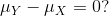
We can never know the true mean or variance of an entire population. Why not? Because we can’t feasibly measure every member of a population. We can never know the true mean blood pressure of all mice, for example, even if all are from one strain, because we can’t afford to buy them all or even find them all. We can never know the true mean blood pressure of all people on a Western diet, for example, because we can’t possibly measure the entire population that’s on a Western diet. If we could measure all people on a Western diet, we really are interested in the difference in means between people on a Western vs. non high fat high sugar diet because we want to know what effect the diet has on people. If there is no difference in means, we can say that there is no effect of diet. If there is a difference in means, we can say that the diet has an effect. The question we are asking can be expressed as:

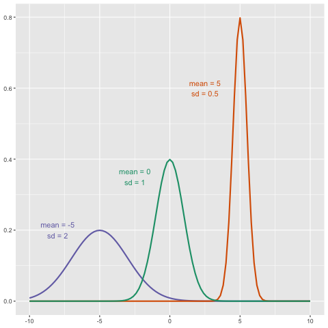
We can even compare more than two means. The three normal curves below help to visualize a question comparing the means of each curve to one of the others.

We also want to know the variance from the mean, so that we have a sense of the spread of measurement around the mean.

In reality we use sample estimates of population parameters. The true population parameters that we are interested in are mean and standard deviation. Here we learn how taking a sample permits us to answer our questions about differences between groups. This is the essence of statistical inference.

Now that we have introduced the idea of a random variable, a null distribution, and a p-value, we are ready to describe the mathematical theory that permits us to compute p-values in practice. We will also learn about confidence intervals and power calculations.

Population parameters

A first step in statistical inference is to understand what population you are interested in. In the mouse weight example, we have two populations: female mice on control diets and female mice on high fat diets, with weight being the outcome of interest. We consider this population to be fixed, and the randomness comes from the sampling. One reason we have been using this dataset as an example is because we happen to have the weights of all the mice of this type. We download this file to our working directory and read in to R:

pheno <- read.csv(file = "../data/mice_pheno.csv")

We can then access the population values and determine, for example, how many we have. Here we compute the size of the control population:

controlPopulation <- filter(pheno, Sex == "F" & Diet == "chow") %>%
  select(Bodyweight) %>% unlist
length(controlPopulation)

[1] 225

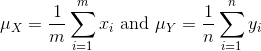
We usually denote these values as x ₁,…,x_m. In this case, m is the number computed above. We can do the same for the high fat diet population:

hfPopulation <- filter(pheno, Sex == "F" & Diet == "hf") %>%  
  select(Bodyweight) %>% unlist
length(hfPopulation)

[1] 200

and denote with y ₁,…,y_n.

We can then define summaries of interest for these populations, such as the mean and variance.

The mean:

# X is the control population
sum(controlPopulation) # sum of the xsubi's

[1] 5376.01

length(controlPopulation) # this equals m

[1] 225

sum(controlPopulation)/length(controlPopulation) # this equals mu sub x

[1] 23.89338

# Y is the high fat diet population
sum(hfPopulation) # sum of the ysubi's

[1] 5253.779

sum(hfPopulation)/length(hfPopulation) # this equals mu sub y

[1] 26.2689

The variance:

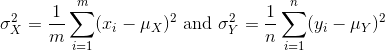
with the standard deviation being the square root of the variance. We refer to such quantities that can be obtained from the population as population parameters. The question we started out asking can now be written mathematically: is μ_Y - μ_X = 0 ?

Although in our illustration we have all the values and can check if this is true, in practice we do not. For example, in practice it would be prohibitively expensive to buy all the mice in a population. Here we learn how taking a sample permits us to answer our questions. This is the essence of statistical inference.

Sample estimates

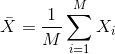
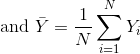
In the previous chapter, we obtained samples of 12 mice from each population. We represent data from samples with capital letters to indicate that they are random. This is common practice in statistics, although it is not always followed. So the samples are X ₁,…,X_M and Y ₁,…,Y_N and, in this case, Ν=Μ=12. In contrast and as we saw above, when we list out the values of the population, which are set and not random, we use lower-case letters.

Since we want to know if μ_Y - μ_X = 0, we consider the sample version: Ȳ-X̄ with:

Note that this difference of averages is also a random variable. Previously, we learned about the behavior of random variables with an exercise that involved repeatedly sampling from the original distribution. Of course, this is not an exercise that we can execute in practice. In this particular case it would involve buying 24 mice over and over again. Here we described the mathematical theory that mathematically relates X̄ to μ_X and Ȳ to μ_Y, that will in turn help us understand the relationship between Ȳ-X̄ and μ_Y - μ_X. Specifically, we will describe how the Central Limit Theorem permits us to use an approximation to answer this question, as well as motivate the widely used t-distribution.

Exercise

We will use the mouse phenotype data. Remove the observations that contain missing values:

pheno <- na.omit(pheno)

Use dplyr to create a vector x with the body weight of all males on the control (chow) diet.
What is this population’s average body weight?

Solution

# Omit observations with missing data
pheno <- na.omit(pheno)

# Create subset of males on chow diet
x <- pheno %>%
  filter(Diet == "chow" & Sex == "M") %>%
  select(Bodyweight) %>%
  unlist

# Calculate mean weight
mean(x)

[1] 30.96381

Set the seed at 1. Take a random sample X of size 25 from x. What is the sample average?

Solution

set.seed(1)
x_sample <- sample(x, 25)
mean(x_sample)

[1] 30.5196

Use dplyr to create a vector y with the body weight of all males on the high fat (hf) diet.
What is this population’s average?

Solution

# Create subset of males on high fat diet
y <- pheno %>%
  filter(Diet == "hf" & Sex == "M") %>%
  select(Bodyweight) %>%
  unlist

# Calculate the mean weight
mean(y)

[1] 34.84793

Set the seed at 1. Take a random sample Y of size 25 from y. What is the sample average?

Solution

set.seed(1)
y_sample <- sample(y, 25)
mean(y_sample)

[1] 35.8036

What is the difference in absolute value between x̄-ȳ and X̄-Ȳ?

Solution

# mu_x - mu_y
pop_mean_diff <- abs(mean(x) - mean(y))
# x-bar - y-bar
sample_mean_diff <- abs(mean(x_sample) - mean(y_sample))
# difference in absolute value between (mu_x - mu_y) - (x-bar - y-bar)
pop_sample_mean_diff <- abs(pop_mean_diff - sample_mean_diff)

pop_sample_mean_diff

[1] 1.399884

Repeat the above for females. Make sure to set the seed to 1 before each sample call. What is the difference in absolute value between x̄-ȳ and X̄-Ȳ?

Solution

x_f <- pheno %>%
    filter(Diet == "chow" & Sex == "F") %>%
    select(Bodyweight) %>%
    unlist
mean(x_f)

[1] 23.89338

set.seed(1)
x_f_sample <- sample(x_f, 25)
mean(x_f_sample)

[1] 24.2528

y_f <- pheno %>%
    filter(Diet == "hf" & Sex == "F") %>%
    select(Bodyweight) %>%
    unlist
mean(y_f)

[1] 26.2689

set.seed(1)
y_f_sample <- sample(y_f, 25)
mean(y_f_sample)

[1] 28.3828

pop_mean_diff_f <- abs(mean(x_f) - mean(y_f))
sample_mean_diff_f <- abs(mean(x_f_sample) - mean(y_f_sample))
pop_sample_mean_diff_f <- abs(pop_mean_diff_f - sample_mean_diff_f)

pop_sample_mean_diff_f

[1] 1.754483

Key Points

• Parameters are measures of populations.

• Statistics are measures of samples drawn from populations.

• Statistical inference is the process of using sample statistics to answer questions about population parameters.