Introduction to scRNA-seq

Overview

Teaching: 10 min
Exercises: 5 min

Questions

• What is the advantages of scRNA-seq?

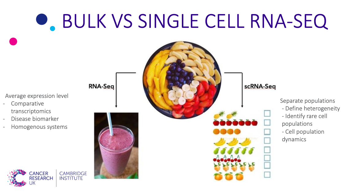
• What is the difference between bulk RNA-seq and scRNA-seq?

Objectives

• Understand the the purpose of using next-generation sequencing (NGS)

• Understand the pitfalls in bulk RNA-seq sequencing, and how can they be overcome

RNA-seq (RNA-sequencing) is a technique that can examine the quantity and sequences of RNA in a sample using next-generation sequencing (NGS). Compared to previous Sanger sequencing- and microarray-based methods, RNA-Seq provides far higher coverage and greater resolution of the dynamic nature of the transcriptome. Beyond quantifying gene expression, the data generated by RNA-Seq facilitate the discovery of novel transcripts, identification of alternatively spliced genes, and detection of allele-specific expression.

Note

We will refer to RNA-seq from now on by bulk RNA-seq to distinguish it from single-cell RNA-seq, which will be introduced later in this episode.

In order to perform bulk RNA-seq studies, samples have to be lysed, and the RNA is extracted. The following steps involve converting a sample of RNA to a cDNA library, which is then sequenced and mapped against a reference genome. The original goal of RNA sequencing was to compare the actual transcript abundance between samples.

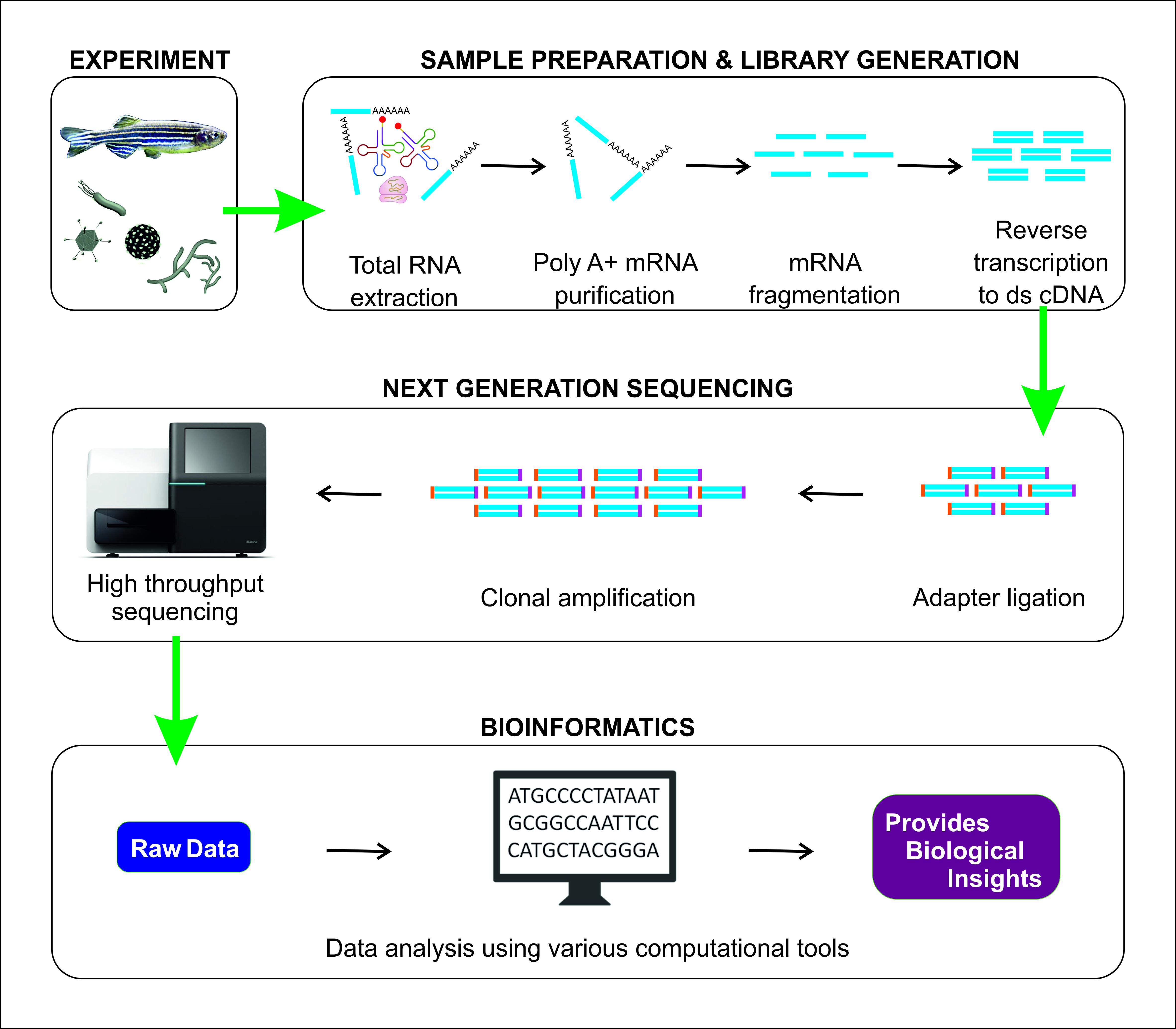
Image is taken from “Sudhagar, A.; Kumar, G.; El-Matbouli, M. Transcriptome Analysis Based on RNA-Seq in Understanding Pathogenic Mechanisms of Diseases and the Immune System of Fish: A Comprehensive Review. Int. J. Mol. Sci. 2018, 19, 245. https://doi.org/10.3390/ijms19010245” under CC-BY license

Question

What is a cDNA library prepration, and why it is used in the bulk RNA-seq?

Solution

RNA is reverse transcribed to cDNA because DNA is more stable and to allow for amplification (which uses DNA polymerases) and leverage more mature DNA sequencing technology. While direct sequencing of RNA molecules is possible, most RNA-Seq experiments are carried out on instruments that sequence DNA molecules due to the technical maturity of commercial instruments designed for DNA-based sequencing. Therefore, cDNA library preparation from RNA is a required step for RNA-Seq. Each cDNA in an RNA-Seq library is composed of a cDNA insert of certain size flanked by adapter sequences, as required for amplification and sequencing on a specific platform.

Pitfall of bulk RNA-seq

• Bulk RNA-seq only provide the average measurement for all the cells. It does not provide insights into the stochastic nature of gene expression. The image below show that although average can be the same, the appearance of the dataset can be vary dramatically which means that average can be misleading and meaningless.

This dataset above has always the same mean (X Mean:54.26, Y Mean: 47.83, X SD:16.76, Y SD:26.93, Corr:-0.06) but varied appearance - Taken from Justin Matejka and George Fitzmaurice (Autodesk Research, Toronto)

• Insufficient for studying heterogeneous systems, e.g. early development studies, complex tissues (brain)

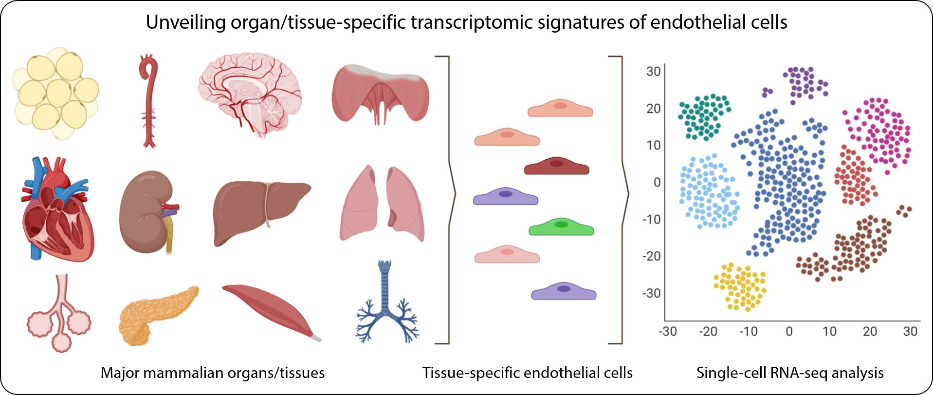
Image is taken from https://doi.org/10.1161/CIRCULATIONAHA.119.041433 under CC-BY license

Therefore, scRNA-seq was introduced to overcome the limitations of bulk RNA-seq.

Question

What do we mean by “stochastic nature of gene expression”?

Solution

It means that there are fluctuations in the abundance of expressed genes at the single-cell level because of the heterogeneity within populations of genetically identical cells.

Kærn, M., Elston, T., Blake, W. et al. Stochasticity in gene expression: from theories to phenotypes. Nat Rev Genet 6, 451–464 (2005). https://doi.org/10.1038/nrg1615

• Even Though cell lines might seem more homogenous than tissue. They undergoes cell cycle heterogeneity, which can’t be taken into account during bulk RNA-seq

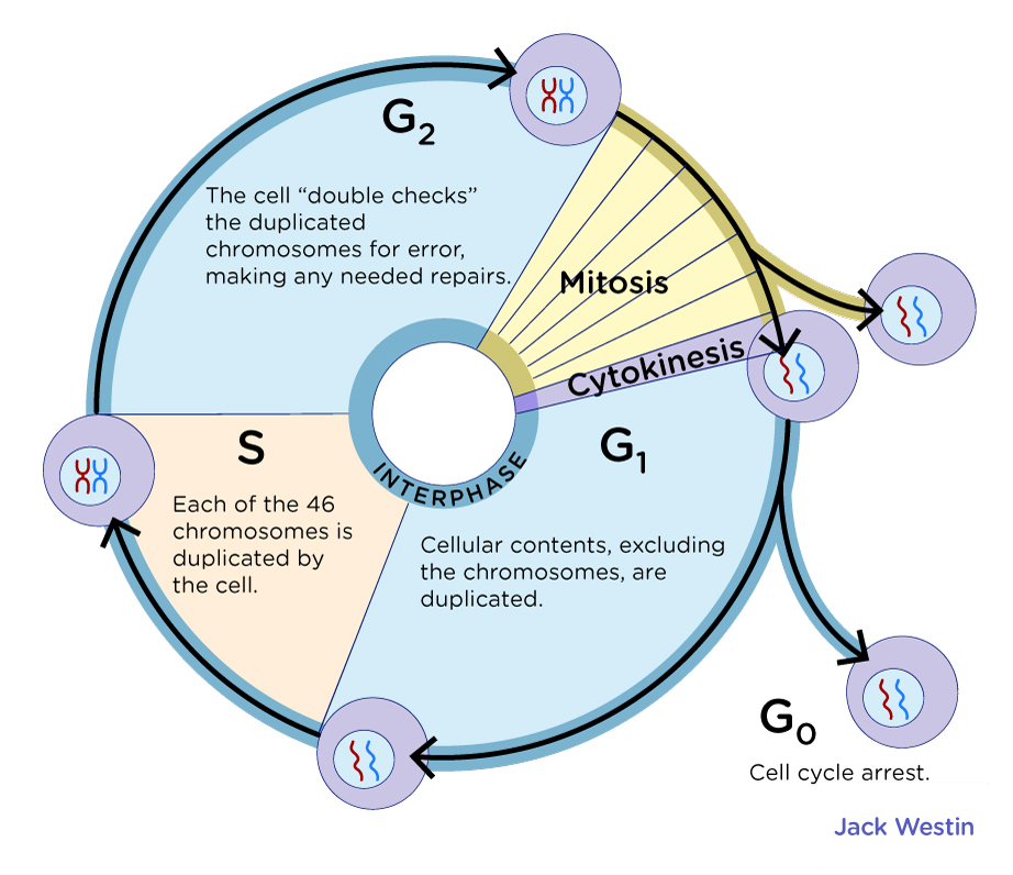
Image is taken from jackwestin.com under CC-BY license

Introduction to single-cell RNA-seq

The main difference between bulk and single-cell RNA-seq (scRNA-seq) is that each sequencing library represents a single cell, instead of a population of cells. Bulk sample analysis is just like putting a fruit salad into a blender - the taste is an average of all ingredients. Analyzing single cells is like tasting each individual piece of fruit to gain a much more nuanced understanding of the composition of the fruit salad Single cell genomics

The advantages of using scRNA-seq

• It allows the measurement of the distribution of expression levels for each gene across a population of cells.
• It also allows to study new biological questions in which cell-specific changes in transcriptome are important, e.g. cell type identification, heterogeneity of cell responses, stochasticity of gene expression, inference of gene regulatory networks across the cells.
• The main advantage of scRNA-seq is that the cellular resolution and the genome-wide scope make it possible to address intractable issues using other methods, e.g. bulk RNA-seq or single-cell RT-qPCR.

However, to analyse scRNA-seq data, novel methods are required, and some of the underlying assumptions for the methods developed for bulk RNA-seq experiments are no longer valid. There are also many different protocols in use, e.g. SMART-seq2 (Picelli et al. 2013), CELL-seq (Hashimshony et al. 2012) and Drop-seq (Macosko et al. 2015), which adds to the complexity of analysing scRNA-seq. In the next episode, we will briefly explore the various experimental methods currently used for scRNA-seq.

Resources Consulted & Recommended Reading

• Mehmet Tekman, Hans-Rudolf Hotz, Daniel Blankenberg, Wendi Bacon, 2021 Pre-processing of 10X Single-Cell RNA Datasets (Galaxy Training Materials). /training-material/topics/transcriptomics/tutorials/scrna-preprocessing-tenx/tutorial.html Online; accessed Tue Apr 06 2021
• Batut et al., 2018 Community-Driven Data Analysis Training for Biology Cell Systems 10.1016/j.cels.2018.05.012

Key Points

• scRNA-seq offers many advantages over bulk RNA-seq

• scRNA-seq requires more pre-processing than bulk RNA-seq

scRNA-seq Workflow

Overview

Teaching: 15 min
Exercises: 5 min

Questions

• What is the standard workflow of scRNA-seq?

Objectives

• Understand the main steps in scRNA-seq experiments.

• Understand the main steps in scRNA-seq data analysis.

• Understand the challanges in scRNA-seq data analysis.

scRNA-Seq Experimental Workflow

Single cell RNA sequencing (scRNA-seq) is a novel technique for extracting more detailed information from genome. Technically, scRNA-seq includes two parts of experimental design and data analysis. As it was mentioned before, scRNA-seq is useful in case of heterogeniety of cells and developmental studies. For example, imagine brain tissue with tens of cell types with tens of different expression profiles. For extracting transcriptome of each cell, it is necessary to isolate each cell from the tissue properly.

Note

A challange in experiment design of scRNA-seq is to isolate cells and prepare a comprehensive library.

Several methods have been developed to overcome this challange from which STRT-seq, SMART-seq, CEL-seq, MARS-seq, Fluidigm C1, CytoSeq, Drop-seq, inDrop, 10x Genomics, SPLiT-seq, sci-RNA-seq, DronC-seq, and Seq-Well can be mentioned. The developmental process of sequencing techniques has been mentioned by Svensson and colleagues.

There is a specific terminology for scRNA-seq which we should know for analysis of data. Lets check them out!

scRNA-seq dictionary

• Unique Molecular Identifiers (UMI): Short random molecular tags which are added to DNA fragments in library preparation process before PCR amplification. UMIs are used to identify input DNA molecules.

• External RNA Controls Consortium (ERCC) spike-in: A short RNA sequence which is used to calibrate measurements of RNA hybridization assays. ERCC spike-ins bind to DNA molecules with matching as control probes.

• Cell Barcode: unique nucleic acid sequences, termed barcodes, which are used to label individual cells, so that they can be tracked through space and time in scRNA-seq.

• Flourescence-activated cell sorting (FACS): A flowcytometry method for cell isolation in which fluorescent tags are used to detect each cell.

• laser capture microdissection (LCM): Cell sorting method under direct microscopic visualization.

Here, you can see the order and construction of reads in scRNA-seq:

Cell barcodes are used to determine each read belongs to which cell and UMI is used for identification of each RNA molecule and enales counting the frequency of reads.

scRNA-Seq Computational Workflow

scRNA-seq raw data includes reads with cell barcode and UMIs. Before alignment of reads to genome, reads can be grouped using cell barcodes and the frequency of each read is estimated per cell per gene using UMIs. After alignment and frequency calculations, we have a gene expression table containing cells represented in the columns and genes represented in the rows. This is what we analyze in scRNA-seq comlutational workflow.

Here You can see the bioinformatics workflow for analysis of scRNA-seq data.

Key Points

• scRNA-seq requires much pre-processing before analysis can be performed.

Pre-processing of scRNA-seq using Cellranger

Overview

Teaching: 15 min
Exercises: 5 min

Questions

• How do pre-process scRNA-seq data using cellranger?

Objectives

• Identify the available tools to preprocess cRNA-seq.

• Understand how to use Cell Ranger.

Dataset:

Expression data from scRNA-seq experiments represent thousands of reads for thousands of cells. Therefore, the data output can be very large and hard to store in your local machine. You will also need higher amounts of memory to analyse.

In this tutorial, We will use Human peripheral blood mononuclear cells (PBMCs) of a healthy female donor aged 25-30 were obtained by 10x Genomics. Libraries were generated from ~16,000 cells (11,996 cells recovered) as described in the Chromium Single Cell 3’ Reagent Kits User Guide (v3.1 Chemistry Dual Index) (CG000315 Rev C) using the Chromium X and sequenced on an Illumina NovaSeq 6000 to a read depth of approximately 40,000 mean reads per cell.

FIXME: Add an image.

Generation of count matrix:

In this part, we will generate the count matrix from the raw sequencing data. After sequencing, the output generated from the sequencing machine will be either output the raw sequencing data as BCL or FASTQ format. Using this raw sequence, we will generate the count matrix.

When using 10X Genomics library preparation method, then the Cell Ranger pipeline is most ideal way to pre-process the data. Make sure that you installed the Cell Ranger version 6.1 (see the instructions). Using cellranger, we can genome mapping, UMI filtering, UMI dedeplication and cell filtering.

FIXME: We need to add image cellranger pipeline where we shows different steps (e.g. extraction, filtering, ..) and also how to correct the naming of the input file

FIXME: Need to subset the dataset for the use only for this part of the lesson and refer to that at the beginning and the end.

In order to align the fastqs to the reference genome and count how many reads per gene per cell. We ca use cellranger count command.

cellranger count --id=bcl \
                   --transcriptome=/opt/refdata-cellranger-GRCh38-3.0.0 \
                   --fastqs=PATH_TO_FASTQ/ \
                   --sample=mysample\
                   --expect-cells=8000

Question

What do you do if your input from sequencing machine is bcl file?

Solution

cellranger wraps the illumina bcl2fastq command into cellranger mkfastq to convert it to fastq files for single-cell RNAseq data.

What is the output of cellranger count?

In the outs folder, and you will find the filtered_feature_bc_matrix folder, which contains 3 files. We can explore these files using ls command.

ls filtered_feature_bc_matrix/
  barcodes.tsv.gz   features.tsv.gz   9 matrix.mtx.gz

We can look into individual files using zcat and head command. The barcodes.tsv.gz should contains all the cell barcodes that passed the cellranger filter.

FIXME: Fix all the names/sequences when you subset the files

zcat barcodes.tsv.gz | head -5
AAAAAAACCCCCCCCC-1
AAAAAAACCCCCCCCC-1
AAAAAAACCCCCCCCC-1
AAAAAAACCCCCCCCC-1
AAAAAAAACCCCCCCCC-1

We can count how many cell/barcodes in barcodes.tsv.gz

zcat barcodes.tsv.gz | wc -l
11544

The second file is the features.tsv.gz, which contains the ENSEMBLE ID and gene symbol

zcat features.tsv.gz | head -5
ENSG00000222222 MPRRCCC     Gene Expression
ENSG00000222222 MPRRCCC Gene Expression
ENSG00000222222 MPRRCCC   Gene Expression
ENSG00000222222 MPRRCCC      Gene Expression
ENSG00000222222 MPRRCCC      Gene Expression

Question

How can you count the genes?

Solution

We can use zcat features.tsv.gz | wc -l to count the number of genes.

The third output is matrix.mtx.gz which is a sparse matrix which contains the non-zero counts. Sparse matrix efficiently save the disk space by only recording the non-zero entries.

FIXME: Add the dimension of the matrix and index of the row (gene) and column(cell) - Figure is very important here.

FIXME: We need a section explain alternative methods such as Alevin (Salmon Alevin + Alevin QC), STARsolo and Kallisto/ BUStools with images

Key Points

• scRNA-seq requires much pre-processing before analysis can be performed.

Quality Control & Normalization

Overview

Teaching: 15 min
Exercises: 5 min

Questions

• What is the aim of normalization?

Objectives

• To understand the structure of expression matrix.

• To use the Scanpy package for normalization.

• To create an object containing expression matrix, barcodes, and cell IDs.

• Understanding the necessity of normalizing counts for accurate comparison between cells.

Generating Expression Metadata

Sequencing centers deliver the results of scRNA-seq in three formats including BCL, fastq, and .mtx. Raw data for scRNA-seq data are received as BCL2 or fastq files. BCL2 files should be converted into FASTQ files using a command line software called bcl2fastq. Analysis of data in FASTQ format includes Quality Control, Trimming, Alignment, Mapping which are mainly similar to bulk RNA-seq analysis and you can find in Data Carpentry Genomics Lessons. Quantification analysis uses statistical analysis and machine learning methods to detect the number of each transcript and count them per cell. Some of the methodologies normalize the counts of transcripts and filter the genes with no significantly different expression levels among which edgeR, DESeq, DESeq2, etc can be mentioned. The output of quantification analysis is a text file containing gene IDs in rows and cell IDs in columns which is called an expression matrix. In this curriculum, we will work on the expression matrix and will apply the analysis steps on it.

Get Data

The dataset which we use for this workshop includes 6 files in .tsv format with information about cell barcodes, metadata, cell IDs and gene IDs and one file in .mtx format which includes the number of RNAs per cell.

Project Directory

scRNA-seq analysis workflow begins with a few files and will produce a lot of files. So it is a big data project and it is useful to manage our files and directories. For this, create a directory called scRNA-seq and four subdirectories called data, scripts, output, and docs.

$ mkdir -p scRNA/{data,docs,output,scripts}.
$ ls
$ cd scRNA/data

As we do for all big data projects, for a better data management in here, we can add the date of files generation at the first part of files names. For example, 2021-09-20-normalization.txt.

Exercise

Discuss your results with your classmate. What are the advantages and disadvantages of file name system suggested? Which system do you suggest for file names which helps for better management of scRNA-seq as a big data project?

Solution

• Advantages: Reproducibility. Easy to track the project progress. Disadvantage: Not all of the collaborators use the same manner for the data management. It makes hard to merge files and data.

Please download dataset using the link in setup (should be linked) into the data directory using the command below:

$ wget -c data-link
$ ls

barcodes.tsv.gz  deng-reads.rds  features.tsv.gz  matrix.mtx.gz  molecules.txt reads.rds  reads.txt  TPs.txt  umi.rds

Preprocessing

The first step using expression matrix is preprocessing divided into two main steps of preprocessing and normalization.

SCANPY

Scanpy is a large scale toolkit for analysis of single-cell gene expression data. The methods for preprocessing, visualization, clustering, pseudotime and trajectory inference, differential expression testing, and simulation of gene regulatory networks are included. The Python-based implementation of SCANPY efficiently deals with data sets of more than one million cells.

You can see that there are different data structures. For this lesson, scanpy is used in combination with pandas and numpy libraries. In the following steps, matplotlib will be needed for visualization, too. For this, the libraries should be imported as below:

$ import scanpy as sc
$ import pandas as pd
$ import numpy as np

Now, configuration settings of scanpy should be performed. Verbosity is an attribute for management of warning messages. The second line is used for creating a log file and the thهrd line is the method for general settings of the graph.

$ sc.settings.verbosity = 3             # verbosity: errors (0), warnings (1), info (2), hints (3)
$ sc.logging.print_header()
$ sc.settings.set_figure_params(dpi=80, facecolor='white')

Which will give you the following output:

scanpy==1.6.0 anndata==0.7.5.dev7+gefffdfb umap==0.4.2 numpy==1.18.1 scipy==1.4.1 pandas==1.0.3 scikit-learn==0.22.1 statsmodels==0.11.0 python-igraph==0.7.1 leidenalg==0.7.0

A file is generated to store the analysis results:

$ results_file = 'write/pbmc3k.h5ad'

Based on the different types of files, it is needed to create an object which contains data of count matrix, annotations, barcodes, etc. The object is called AnnData. AnnData stores data in its special format called h5ad. The object named as adata is created using the code below:

$ adata = sc.read_10x_mtx(
$   'data/filtered_gene_bc_matrices/hg19/',  # the directory with the `.mtx` file
$   var_names='gene_symbols',                # use gene symbols for the variable names (variables-axis index)
$   cache=True)                              # write a cache file for faster subsequent reading

sc.read_10x_mtx is used for reading expression data matrix. hg19 is the directory where .mtx file is stored. var_names is set to use gene_symbols. cahe=True is the code to write a cache file for faster subsequent reading.

... reading from cache file cache/data-filtered_gene_bc_matrices-hg19-matrix.h5ad

Now, it is possible to check out the contents of adata object:

$ adata

AnnData object with n_obs × n_vars = 2700 × 32738
    var: 'gene_ids'

The output shows that there are 2700 columns containing observations and 32738 rows including the variables with gene_id information in the reads count expression matrix.

Preprocessing & Normalization

Expression matrix contains all the genes and their expression levels. As the first step of filtering, it is possible to find the first twenty genes with highest expression levels using the code below:

$ sc.pl.highest_expr_genes(adata, n_top=20, )

Figure should be added.

Usually, filtering is applied on two dimensions of the expression matrix: cells and genes. For this, scanpy includes four important filteration functions included in pp (preprocessing) module: filter_cells, filter_genes, and filter_highly_variable_genes, and normalize_total. Each function has parameter. Here, some challenges are required!

Exercise

Which one of the following options can descripe min_counts better?

1) Minimum number of genes required for a count to pass filtering. 2) Minimum number of counts required for a cell to pass filtering. 3) Minimum number of counts required for a gene to pass filtering. 4) Minimum number of cells required to pass filtering.

Solution

Option No.2.

In the same way, it is possible to explain min_genes, min_cells, max_counts, and max_genes, etc,.

Exercise

Which one of the following options can descripe n_top_genes better?

1) Number of highly-variable genes to remove. 2) Number of highly expressed genes to keep. 3) Number of highly-variable genes to keep. Mandatory if flavor=’seurat_v3’. 4) Number of highly expressed genes to remove.

Solution

Option No.3.

Now, basic and actual filtering can be performed.

$ sc.pp.filter_cells(adata, min_genes=200)
$ sc.pp.filter_genes(adata, min_cells=3)

filtered out 19024 genes that are detected in less than 3 cells

One main step for quality control of expression matrix is to achieve the information about the proportion of mitochondrial genes.

Mitochondiral genes a challenge for scRNA-seq

Cells with poor quality in scRNA-sq contain high proportions of mitochondrial genes. These cells are assumed to be discarded before entering into the droplet. Not filtering mitochondrial genes can cause formation a separate cluster in the further steps.

Quality control is performed using calculate_qc_metrics function in pp module of scanpy using the code below:

$ adata.var['mt'] = adata.var_names.str.startswith('MT-')  
$ sc.pp.calculate_qc_metrics(adata, qc_vars=['mt'], percent_top=None, log1p=False, inplace=True)

This code annotates the group of mitochondrial genes as ‘mt’.

Now, visualization is possible.

Violin Plots

• Violin plots are used for visualization of quality control results in scRNA-seq.
• The number of genes expressed in the count matrix, the total counts per cell, and the percentage of counts in mitochondrial genes.
• These plots are similar to box plots with addition of the probability density of the data at different values.

$ sc.pl.violin(adata, ['n_genes_by_counts', 'total_counts', 'pct_counts_mt'],
             jitter=0.4, multi_panel=True)

The figures should be added.

Scatter plots are applied to visualize data after removal of mitochondrial genes with very high level of expression.

$ sc.pl.scatter(adata, x='total_counts', y='pct_counts_mt')
$ sc.pl.scatter(adata, x='total_counts', y='n_genes_by_counts')

The figures should be added.

The results of filters are applied to splice AnnData object.

$ adata = adata[adata.obs.n_genes_by_counts < 2500, :]
$ adata = adata[adata.obs.pct_counts_mt < 5, :]

Total-count normalize (library-size correct) is used to make counts comparable among cells. Using this method, the data matrix contains 10,000 reads per cell.

$ sc.pp.normalize_total(adata, target_sum=1e4)

The process takes a few seconds …

normalizing counts per cell
    finished (0:00:00)

Logartimaize data:

$ sc.pp.log1p(adata)

And, identify highly-variable genes:

$ sc.pp.highly_variable_genes(adata, min_mean=0.0125, max_mean=3, min_disp=0.5)

highly_variable_genes function expects normalized and logarithmized data and the variation in genes expression level are rated using the normalized variance of count number. Highly variable gene (HVG) is an important parameter in scRNA-seq that helps to find the genes contribute strongly to cell-to-cell variation within a homogeneous cell population, such as a population of embryonic stem cells.

extracting highly variable genes
    finished (0:00:00)
--> added
    'highly_variable', boolean vector (adata.var)
    'means', float vector (adata.var)
    dispersions', float vector (adata.var)
    'dispersions_norm', float vector (adata.var)

Visualizing the HVGs:

$ sc.pl.highly_variable_genes(adata)

The figure should be added.

Key Points

• scRNA-seq requires much pre-processing before analysis can be performed.

Trimming and Filtering

Overview

Teaching: 30 min
Exercises: 25 min

Questions

• How can I get rid of sequence data that doesn’t meet my quality standards?

Objectives

• Clean FASTQ reads using Trimmomatic.

• Select and set multiple options for command-line bioinformatic tools.

• Write for loops with two variables.

Cleaning Reads

In the previous episode, we took a high-level look at the quality of each of our samples using FastQC. We visualized per-base quality graphs showing the distribution of read quality at each base across all reads in a sample and extracted information about which samples fail which quality checks. Some of our samples failed quite a few quality metrics used by FastQC. This doesn’t mean, though, that our samples should be thrown out! It’s very common to have some quality metrics fail, and this may or may not be a problem for your downstream application. For our variant calling workflow, we will be removing some of the low quality sequences to reduce our false positive rate due to sequencing error.

We will use a program called Trimmomatic to filter poor quality reads and trim poor quality bases from our samples.

Trimmomatic Options

Trimmomatic has a variety of options to trim your reads. If we run the following command, we can see some of our options.

Key Points

• The options you set for the command-line tools you use are important!

• Data cleaning is an essential step in a genomics workflow.