Finetuning LLMs
Overview
Teaching: 60 min
Exercises: 60 minQuestions
How can I fine-tune preexisting LLMs for my own research?
How do I pick the right data format?
How do I create my own labels?
How do I put my data into a model for finetuning?
How do I evaluate success at my task?
Objectives
Examine CONLL2003 data.
Learn about Label Studio.
Learn about finetuning a BERT model.
Setup
If you are running this lesson on Google Colab, it is strongly recommended that you enable GPU acceleration. If you are running locally without CUDA, you should be able to run most of the commands, but training will take a long time and you will want to use the pretrained model when using it.
To enable GPU, click “Edit > Notebook settings” and select GPU. If enabled, this command will return a status window and not an error:
!nvidia-smi
Thu Mar 28 20:50:47 2024
+---------------------------------------------------------------------------------------+
| NVIDIA-SMI 535.104.05             Driver Version: 535.104.05   CUDA Version: 12.2     |
|-----------------------------------------+----------------------+----------------------+
| GPU  Name                 Persistence-M | Bus-Id        Disp.A | Volatile Uncorr. ECC |
| Fan  Temp   Perf          Pwr:Usage/Cap |         Memory-Usage | GPU-Util  Compute M. |
|                                         |                      |               MIG M. |
|=========================================+======================+======================|
|   0  Tesla T4                       Off | 00000000:00:04.0 Off |                    0 |
| N/A   64C    P8              11W /  70W |      0MiB / 15360MiB |      0%      Default |
|                                         |                      |                  N/A |
+-----------------------------------------+----------------------+----------------------+

+---------------------------------------------------------------------------------------+
| Processes:                                                                            |
|  GPU   GI   CI        PID   Type   Process name                            GPU Memory |
|        ID   ID                                                             Usage      |
|=======================================================================================|
|  No running processes found                                                           |
+---------------------------------------------------------------------------------------+
These installation commands will take time to run. Begin them now.
!pip install transformers datasets evaluate seqeval
Finetuning LLMs
In 2017, a revolutionary breakthrough for NLP occurred. A new type of hidden layer for neural networks called Transfomers were invented. Transformers made processing huge amounts of data feasible for the first time.
Large Language Models, or LLMs, were the result. LLMs are the current state of the art when it comes to many tasks, and although LLMs can differ, they are mostly based on a similar architecture to one another. We will be looking at an influential LLM called BERT.
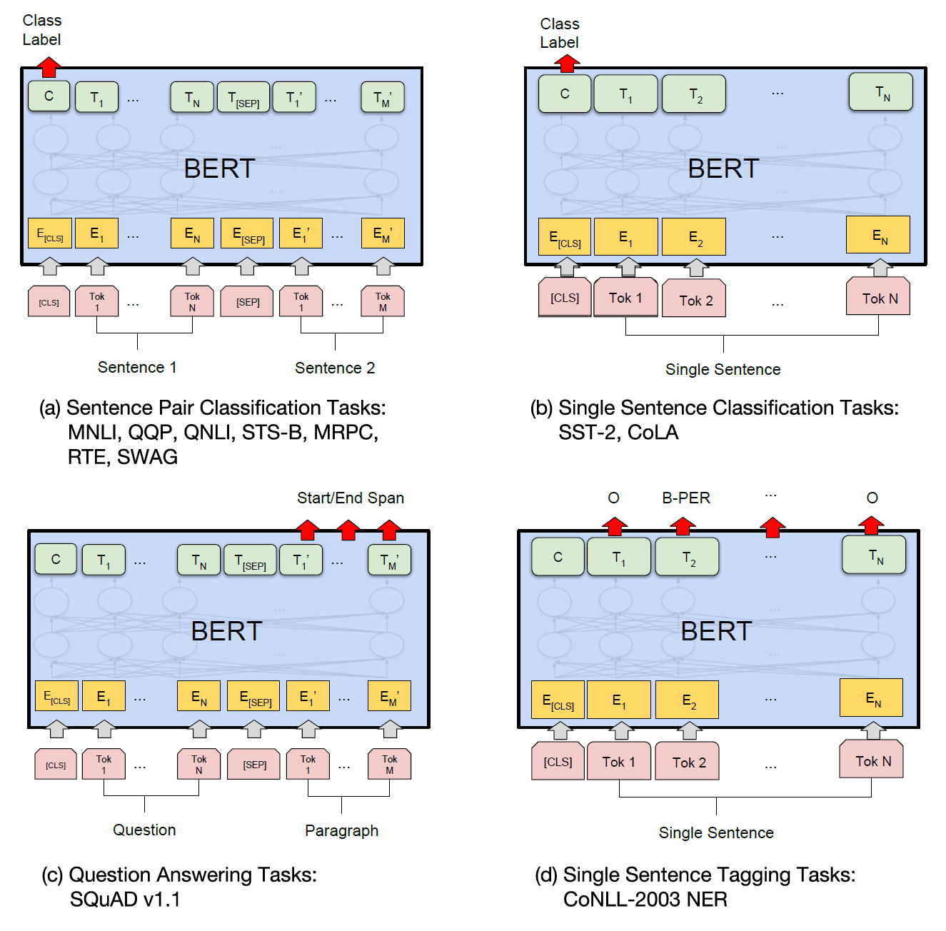
Training these models from scratch requires a huge amount of data and compute power. The majority of work is done for the many hidden layers of the model. However, by tweaking only the output layer, BERT can effectively perform many tasks with a minimal amount of data. This process of adapting an LLM is called fine-tuning.
Because of this, we will not be writing the code for this lesson from scratch. Rather, this lesson will focus on creating our own data, adapting existing code and modifying it to achieve the task we want to accomplish.
Using Existing Model- DistilBERT
We will be using a miniture LLM called DistilBERT for this lesson. We are using the “uncased” version of distilbert, which removes capitalization.
Much like many of our models, DistilBERT is available through HuggingFace. https://huggingface.co/docs/transformers/model_doc/distilbert
Let’s start by importing the library, and importing both the pretrained model and the tokenizer that BERT uses.
from transformers import AutoTokenizer, AutoModelForTokenClassification
from transformers import pipeline

tokenizer = AutoTokenizer.from_pretrained("Davlan/distilbert-base-multilingual-cased-ner-hrl")
model = AutoModelForTokenClassification.from_pretrained("Davlan/distilbert-base-multilingual-cased-ner-hrl")
#The aggregation strategy combines all of the tokens with a given label. Useful when our tokenizer uses subword tokens.
nlp = pipeline("ner", model=model, tokenizer=tokenizer, aggregation_strategy='simple')
Next, we’ll use the tokenizer to preprocess our example sentence.
example = "Nader Jokhadar had given Syria the lead with a well-struck header in the seventh minute."
ner_results = nlp(example)
for result in ner_results:
  print(result)
{'entity_group': 'PER', 'score': 0.9993166, 'word': 'Nader Jokhadar', 'start': 0, 'end': 14}
{'entity_group': 'LOC', 'score': 0.99975127, 'word': 'Syria', 'start': 25, 'end': 30}
LLMs are highly performant at not just one, but a variety of tasks. And there are many versions of LLMs, designed to perform well on a variety of tasks available on HuggingFace.
We could use this existing model for research purposes as is. We might use an existing NER model to find examples of the most common locations in a set of fiction. You could categorize product reviews as positive or negative automatically using sentiment analysis. You could automatically translate documents from one language to another.
There are many possible tasks that LLMs can handle!
Why Fine Tune?
Given that there are many many prebuilt models for BERT, why would you want to go through the trouble of fine tuning your own?
LLM’s are very robust. They aren’t just capable of doing tasks other people have already trained them for. LLMs can also do specific and novel tasks you might want to accomplish as part of research!
Imagine using a LLM to classify a group of documents using training data you create. Or imagine an LLM pulling out specific types of words based on examples you provide. LLM’s can be trained to do these specific tasks fairly well, without needing terabytes of data to do so.
Let’s take a look on how we fine tune an LLM on a novel task by walking through an example.
The Interpretive Loop
To fine-tune, we will walk through all of the steps of our interpretive loop diagram. Let’s take a look at our diagram once more:
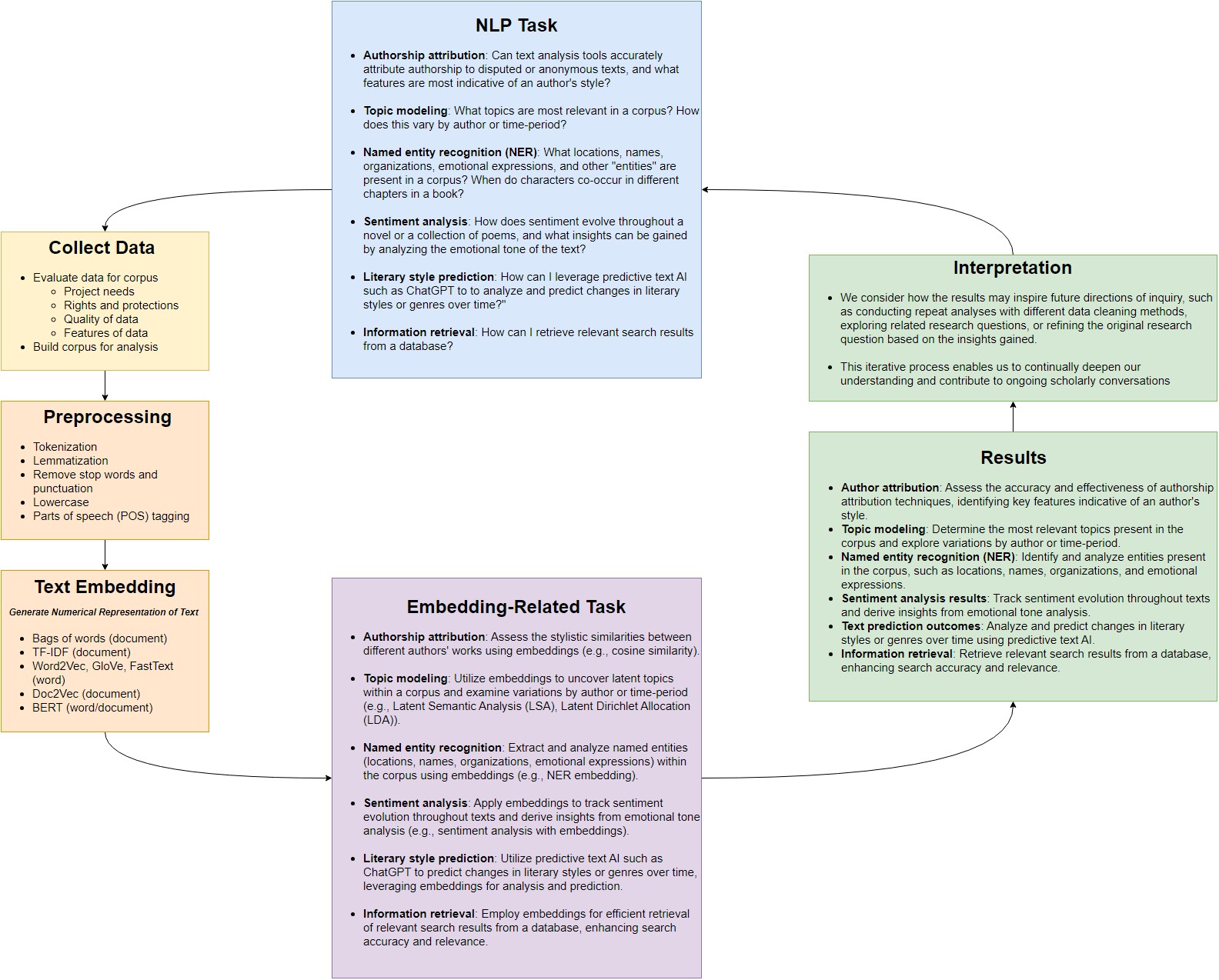
If no existing model does a given task, we can fine-tune a LLM to do it. How do we start? We’re going to create versions of all the items listed in our diagram.
We need the following:
- A task, so we can find a model and LLM pipeline to finetune.
- A dataset for our task, properly formatted in a way BERT can interpret.
- A tokenizer and helpers to preprocess our data in a way BERT expects.
- A model that has been pretrained on millions of documents for us. We will only fine-tune this model, not recreate it from scratch.
- A trainer to fine-tune our model to perform our task.
- A set of metrics so that we can evaluate how well our model performs.
The final product of all this work will be a fine-tuned model that classifies all the elements of reviews that we want. Let’s get started!
NLP task
The first thing we can do is identify our task. Suppose our research question is to look carefully at different elements of restaurant reviews. We want to classify different elements of restaurant reviews, such as amenities, locations, ratings, cuisine types and so on using an LLM.
Our task here is Token Classification, or more specifically, Named Entity Recognition. Classifying tokens will enable us to pull out categories that are of interest to us.
The standard set of Named Entity Recognition labels is designed to be broad: people, organizations and so on. However, it doesn’t have to be. We can define our own entities of interest and have our model search for them.
Now that we have an idea of what we’re aiming to do, lets look at some of the LLMs provided by HuggingFace that perform this activity. HuggingFace hosts many instructional Colab notebooks available at: https://huggingface.co/docs/transformers/notebooks.
We can find an example of Token Classification using PyTorch there. This document will be the basis for our code.
Examining Working Example
Looking at the notebook, we can get an idea of how it functions and adapt it for our own purposes.
- The existing model it uses is a compressed version of BERT, “distilbert.” While not as accurate as the full BERT model, it is smaller and easier to fine tune. We’ll use this model as well.
- The existing dataset for our task is something called “conll2003”. We will want to look at this and replace it with our own data, taking care to copy the formatting of existing data.
- The existing tokenizer requires a special helper method called an aligner. We will copy this directly.
- The existing model that we will tweak to accomplish our task.
- A trainer, which will largely use existing parameters. We will need to tweak our output labels for our new data.
- The existing metrics will be fine, but we have to feed them into our trainer.
Creating training data
It’s a good idea to pattern your data output based on what the model is expecting. You will need to make adjustments, but if you have selected a model that is appropriate to the task you can reuse most of the code already in place. We’ll start by installing our dependencies.
Now, let’s take a look at the example data from the dataset used in the example. The dataset used is called the CoNLL2003 dataset.
from datasets import load_dataset, load_metric

ds = load_dataset("conll2003", trust_remote_code=True)
print(ds)
DatasetDict({
    train: Dataset({
        features: ['id', 'tokens', 'pos_tags', 'chunk_tags', 'ner_tags'],
        num_rows: 14041
    })
    validation: Dataset({
        features: ['id', 'tokens', 'pos_tags', 'chunk_tags', 'ner_tags'],
        num_rows: 3250
    })
    test: Dataset({
        features: ['id', 'tokens', 'pos_tags', 'chunk_tags', 'ner_tags'],
        num_rows: 3453
    })
})
We can see that the CONLL dataset is split into three sets- training data, validation data, and test data. Training data should make up about 80% of your corpus and is fed into the model to fine tune it. Validation data should be about 10%, and is used to check how the training progress is going as the model is trained. The test data is about 10% withheld until the model is fully trained and ready for testing, so you can see how it handles new documents that the model has never seen before.
Let’s take a closer look at a record in the train set so we can get an idea of what our data should look like. The NER tags are the ones we are interested in, so lets print them out and take a look. We’ll also select the dataset and then an index for the document to look at an example.
traindoc = ds["train"][0]
conll_tags = ds["train"].features[f"ner_tags"].feature.names

print(traindoc['tokens'])
print(traindoc['ner_tags'])
print(conll_tags)
print()

for token, ner_tag in zip(traindoc['tokens'], traindoc['ner_tags']):
  print(token+" "+conll_tags[ner_tag])
['EU', 'rejects', 'German', 'call', 'to', 'boycott', 'British', 'lamb', '.']
[3, 0, 7, 0, 0, 0, 7, 0, 0]
['O', 'B-PER', 'I-PER', 'B-ORG', 'I-ORG', 'B-LOC', 'I-LOC', 'B-MISC', 'I-MISC']

EU B-ORG
rejects O
German B-MISC
call O
to O
boycott O
British B-MISC
lamb O
. O
Each document has it’s own ID number. We can see that the tokens are a list of words in the document. For each word in the tokens, there are a series of numbers. Those numbers correspond to the labels in the database. Based on this, we can see that the EU is recognized as an ORG and the terms “German” and “British” are labelled as MISC.
These datasets are loaded using specially written loading scripts. We can look at this script by searching for the ‘conll2003’ in huggingface and selecting “Files”. The loading script is always named after the dataset. In this case it is “conll2003.py”.
https://huggingface.co/datasets/conll2003/blob/main/conll2003.py
Opening this file up, we can see that a zip file is downloaded and text files are extracted. We can manually download this ourselves if we would really like to take a closer look. For the sake of convienence, the example we looked just looked at is reproduced below:
"""
-DOCSTART- -X- -X- O

EU NNP B-NP B-ORG
rejects VBZ B-VP O
German JJ B-NP B-MISC
call NN I-NP O
to TO B-VP O
boycott VB I-VP O
British JJ B-NP B-MISC
lamb NN I-NP O
. . O O
"""
'\n-DOCSTART- -X- -X- O\n\nEU NNP B-NP B-ORG\nrejects VBZ B-VP O\nGerman JJ B-NP B-MISC\ncall NN I-NP O\nto TO B-VP O\nboycott VB I-VP O\nBritish JJ B-NP B-MISC\nlamb NN I-NP O\n. . O O\n'
This is a simple format, similar to a CSV. Each document is seperated by a blank line. The token we look at is first, then space seperated tags for POS, chunk_tags and NER tags. Many of the token classifications use BIO tagging, which specifies that “B” is the beginning of a tag, “I” is inside a tag, and “O” means that the token outside of our tagging schema.
So, now that we have an idea of what the HuggingFace models expect, let’s start thinking about how we can create our own set of data and labels.
Tagging a dataset
Most of the human time spent training a model will be spent pre-processing and labelling data. If we expect our model to label data with an arbitrary set of labels, we need to give it some idea of what to look for. We want to make sure we have enough data for the model to perform at a good enough degree of accuracy for our purpose. Of course, this number will vary based on what level of performance is “good enough” and the difficulty of the task. While there’s no set number, a set of approximately 100,000 tokens is enough to train many NER tasks.
Fortunately, software exists to help streamline the tagging process. One open source example of tagging software is Label Studio. However, it’s not the only option, so feel free to select a data labelling software that matches your preferences or needs for a given project. An online demo of Label Studio is available here: https://labelstud.io/playground. It’s also possible to install locally.
Select “Named Entity Recognition” as the task to see what the interface would look like if we were doing our own tagging. We can define our own labels by copying in the following code (minus the quotations):
"""
<View>
  <Labels name="label" toName="text">
    <Label value="Amenity" background="red"/>
    <Label value="Cuisine" background="darkorange"/>
    <Label value="Dish" background="orange"/>
    <Label value="Hours" background="green"/>
    <Label value="Location" background="darkblue"/>
    <Label value="Price" background="blue"/>
    <Label value="Rating" background="purple"/>
    <Label value="Restaurant_Name" background="#842"/>
  </Labels>

  <Text name="text" value="$text"/>
</View>
"""
'\n<View>\n <Labels name="label" toName="text">\n <Label value="Amenity" background="red"/>\n <Label value="Cuisine" background="darkorange"/>\n <Label value="Dish" background="orange"/>\n <Label value="Hours" background="green"/>\n <Label value="Location" background="darkblue"/>\n <Label value="Price" background="blue"/>\n <Label value="Rating" background="purple"/>\n <Label value="Restaurant_Name" background="#842"/>\n </Labels>\n\n <Text name="text" value="$text"/>\n</View>\n'
In Label Studio, labels can be applied by hitting a number on your keyboard and highlighting the relevant part of the document. Try doing so on our example text and looking at the output.
Once done, we will have to export our files for use in our model. Label Studio supports a number of different types of labelling tasks, so you may want to use it for tasks other than just NER.
One additional note: There is a github project for direct integration between label studio and HuggingFace available as well. Given that the task selected may vary on the model and you may not opt to use Label Studio for a given project, we will simply point to this project as a possible resource (https://github.com/heartexlabs/label-studio-transformers) rather than use it in this lesson.
Export to desired format
So, let’s say you’ve finished your tagging project. How do we get these labels out of label studio and into our model?
Label Studio supports export into many formats, including one called CoNLL2003. This is the format our test dataset is in. It’s a space seperated CSV, with words and their tags.
We’ll skip the export step as well, as we already have a prelabeled set of tags in a similar format published by MIT. For more details about supported export formats consult the help page for Label Studio here: https://labelstud.io/guide/export.html
At this point, we’ve got all the labelled data we want. We now need to load our dataset into HuggingFace and then train our model. The following code will be largely based on the example code from HuggingFace, substituting in our data for the CoNLL data.
Loading our custom dataset
Let’s import our carpentries files and helper methods first, as they contain our data and a loading script.
# Run this cell to mount your Google Drive.
from google.colab import drive
drive.mount('/content/drive')
# pip install necessary to access parse module (called from helpers.py)
!pip install parse
Finally, lets make our own tweaks to the HuggingFace colab notebook. We’ll start by importing some key metrics.
import datasets
from datasets import load_dataset, Features
The HuggingFace example uses CONLL 2003 dataset.
All datasets from huggingface are loaded using scripts. Datasets can be defined from a JSON or csv file (see the Datasets documentation) but selecting CSV will by default create a new document for every token and NER tag and will not load the documents correctly. So we will use a tweaked version of the Conll loading script instead. Let’s take a look at the regular Conll script first:
https://huggingface.co/datasets/conll2003/tree/main
The loading script is the python file. Usually the loading script is named after the dataset in question. There are a couple of things we want to change-
- We want to tweak the metadata with citations to reflect where we got our data. If you created the data, you can add in your own citation here.
- We want to define our own categories for NER_TAGS, to reflect our new named entities.
- The order for our tokens and NER tags is flipped in our data files.
- Delimiters for our data files are tabs instead of spaces.
- We will replace the method names with ones appropriate for our dataset.
Those modifications have been made in our mit_restaurants.py file. Let’s briefly take a look at that file before we proceed with the huggingface script. Again, these are modifications, not working from scratch.
HuggingFace Code
Now that we have a modified huggingface script, let’s load our data.
ds = load_dataset("/content/drive/MyDrive/Colab Notebooks/text-analysis/code/mit_restaurants.py", trust_remote_code=True)
/usr/local/lib/python3.10/dist-packages/datasets/load.py:926: FutureWarning: The repository for mit_restaurants contains custom code which must be executed to correctly load the dataset. You can inspect the repository content at /content/drive/MyDrive/Colab Notebooks/text-analysis/code/mit_restaurants.py
You can avoid this message in future by passing the argument `trust_remote_code=True`.
Passing `trust_remote_code=True` will be mandatory to load this dataset from the next major release of `datasets`.
  warnings.warn(
How does our dataset compare to the CONLL dataset? Let’s look at a record and compare.
ds
DatasetDict({
    train: Dataset({
        features: ['id', 'tokens', 'ner_tags'],
        num_rows: 7660
    })
    validation: Dataset({
        features: ['id', 'tokens', 'ner_tags'],
        num_rows: 815
    })
    test: Dataset({
        features: ['id', 'tokens', 'ner_tags'],
        num_rows: 706
    })
})
label_list = ds["train"].features[f"ner_tags"].feature.names
label_list
['O',
 'B-Amenity',
 'I-Amenity',
 'B-Cuisine',
 'I-Cuisine',
 'B-Dish',
 'I-Dish',
 'B-Hours',
 'I-Hours',
 'B-Location',
 'I-Location',
 'B-Price',
 'I-Price',
 'B-Rating',
 'I-Rating',
 'B-Restaurant_Name',
 'I-Restaurant_Name']
Our data looks pretty similar to the CONLL data now. This is good since we can now reuse many of the methods listed by HuggingFace in their Colab notebook.
Preprocessing the data
We start by defining some variables that HuggingFace uses later on.
import torch

task = "ner" # Should be one of "ner", "pos" or "chunk"
model_checkpoint = "distilbert-base-uncased"
batch_size = 16
device = torch.device("cuda" if torch.cuda.is_available() else "cpu")
Next, we create our special BERT tokenizer.
from transformers import AutoTokenizer
tokenizer = AutoTokenizer.from_pretrained(model_checkpoint)
example = ds["train"][4]
tokenized_input = tokenizer(example["tokens"], is_split_into_words=True)
tokens = tokenizer.convert_ids_to_tokens(tokenized_input["input_ids"])
print(tokens)
['[CLS]', 'a', 'great', 'lunch', 'spot', 'but', 'open', 'till', '2', 'a', 'm', 'pass', '##im', '##s', 'kitchen', '[SEP]']
Since our words are broken into just words, and the BERT tokenizer sometimes breaks words into subwords, we need to retokenize our words. We also need to make sure that when we do this, the labels we created don’t get misaligned. More details on these methods are available through HuggingFace, but we will simply use their code to do this.
word_ids = tokenized_input.word_ids()
aligned_labels = [-100 if i is None else example[f"{task}_tags"][i] for i in word_ids]
label_all_tokens = True
def tokenize_and_align_labels(examples):
    tokenized_inputs = tokenizer(examples["tokens"], truncation=True, is_split_into_words=True)

    labels = []
    for i, label in enumerate(examples[f"{task}_tags"]):
        word_ids = tokenized_inputs.word_ids(batch_index=i)
        previous_word_idx = None
        label_ids = []
        for word_idx in word_ids:
            # Special tokens have a word id that is None. We set the label to -100 so they are automatically
            # ignored in the loss function.
            if word_idx is None:
                label_ids.append(-100)
            # We set the label for the first token of each word.
            elif word_idx != previous_word_idx:
                label_ids.append(label[word_idx])
            # For the other tokens in a word, we set the label to either the current label or -100, depending on
            # the label_all_tokens flag.
            else:
                label_ids.append(label[word_idx] if label_all_tokens else -100)
            previous_word_idx = word_idx

        labels.append(label_ids)

    tokenized_inputs["labels"] = labels
    return tokenized_inputs
tokenized_datasets = ds.map(tokenize_and_align_labels, batched=True)
print(tokenized_datasets)
Map:   0%|          | 0/815 [00:00<?, ? examples/s]


DatasetDict({
    train: Dataset({
        features: ['id', 'tokens', 'ner_tags', 'input_ids', 'attention_mask', 'labels'],
        num_rows: 7660
    })
    validation: Dataset({
        features: ['id', 'tokens', 'ner_tags', 'input_ids', 'attention_mask', 'labels'],
        num_rows: 815
    })
    test: Dataset({
        features: ['id', 'tokens', 'ner_tags', 'input_ids', 'attention_mask', 'labels'],
        num_rows: 706
    })
})
The preprocessed features we’ve just added will be the ones used to actually train the model.
Fine-tuning the model
Now that our data is ready, we can download the pretrained LLM model. Since our task is token classification, we use the AutoModelForTokenClassification class. Before we do though, we want to specify the mapping for ids and labels to our model so it does not simply return CLASS_1, CLASS_2 and so on.
id2label = {
    0: "O",
    1: "B-Amenity",
    2: "I-Amenity",
    3: "B-Cuisine",
    4: "I-Cuisine",
    5: "B-Dish",
    6: "I-Dish",
    7: "B-Hours",
    8: "I-Hours",
    9: "B-Location",
    10: "I-Location",
    11: "B-Price",
    12: "I-Price",
    13: "B-Rating",
    14: "I-Rating",
    15: "B-Restaurant_Name",
    16: "I-Restaurant_Name",
}

label2id = {
    "O": 0,
    "B-Amenity": 1,
    "I-Amenity": 2,
    "B-Cuisine": 3,
    "I-Cuisine": 4,
    "B-Dish": 5,
    "I-Dish": 6,
    "B-Hours": 7,
    "I-Hours": 8,
    "B-Location": 9,
    "I-Location": 10,
    "B-Price": 11,
    "I-Price": 12,
    "B-Rating": 13,
    "I-Rating": 14,
    "B-Restaurant_Name": 15,
    "I-Restaurant_Name": 16,
}
from transformers import AutoModelForTokenClassification, TrainingArguments, Trainer

model = AutoModelForTokenClassification.from_pretrained(model_checkpoint, id2label=id2label, label2id=label2id, num_labels=len(label_list)).to(device)
Some weights of DistilBertForTokenClassification were not initialized from the model checkpoint at distilbert-base-uncased and are newly initialized: ['classifier.bias', 'classifier.weight']
You should probably TRAIN this model on a down-stream task to be able to use it for predictions and inference.
The warning is telling us we are throwing away some weights. We’re training our model, so we should be fine.
##Configuration Arguments
Next, we configure our trainer. The are lots of settings here but the defaults are fine. More detailed documentation on what each of these mean are available through Huggingface: TrainingArguments,
model_name = model_checkpoint.split("/")[-1]
args = TrainingArguments(
    #f"{model_name}-finetuned-{task}",
    f"{model_name}-carpentries-restaurant-ner",
    learning_rate=2e-5,
    per_device_train_batch_size=batch_size,
    per_device_eval_batch_size=batch_size,
    num_train_epochs=3,
    weight_decay=0.01,
    report_to="none",
    eval_strategy="epoch",
    save_strategy="epoch",
    load_best_model_at_end=True,
    push_to_hub=False, #You can have your model automatically pushed to HF if you uncomment this and log in.
)
Collator
One finicky aspect of the model is that all of the inputs have to be the same size. When the sizes do not match, something called a data collator is used to batch our processed examples together and pad them to the same size.
from transformers import DataCollatorForTokenClassification

data_collator = DataCollatorForTokenClassification(tokenizer)
Metrics
The last thing we want to define is the metric by which we evaluate how our model did. We will use seqeval. The metric used will vary based on the task- make sure to check the huggingface notebooks for the appropriate metric for a given task.
import evaluate

seqeval = evaluate.load("seqeval")
Post Processing
Per HuggingFace- we need to do a bit of post-processing on our predictions. The following function and description is taken directly from HuggingFace. The function does the following:
- Selected the predicted index (with the maximum logit) for each token
- Converts it to its string label
- Ignore everywhere we set a label of -100
import numpy as np

def compute_metrics(p):
    predictions, labels = p
    predictions = np.argmax(predictions, axis=2)

    # Remove ignored index (special tokens)
    true_predictions = [
        [label_list[p] for (p, l) in zip(prediction, label) if l != -100]
        for prediction, label in zip(predictions, labels)
    ]
    true_labels = [
        [label_list[l] for (p, l) in zip(prediction, label) if l != -100]
        for prediction, label in zip(predictions, labels)
    ]

    results = metric.compute(predictions=true_predictions, references=true_labels)
    return {
        "precision": results["overall_precision"],
        "recall": results["overall_recall"],
        "f1": results["overall_f1"],
        "accuracy": results["overall_accuracy"],
    }
Finally, after all of the preparation we’ve done, we’re ready to create a Trainer to train our model.
trainer = Trainer(
    model,
    args,
    train_dataset=tokenized_datasets["train"],
    eval_dataset=tokenized_datasets["validation"],
    data_collator=data_collator,
    tokenizer=tokenizer,
    compute_metrics=compute_metrics,
)
/usr/local/lib/python3.10/dist-packages/accelerate/accelerator.py:432: FutureWarning: Passing the following arguments to `Accelerator` is deprecated and will be removed in version 1.0 of Accelerate: dict_keys(['dispatch_batches', 'split_batches', 'even_batches', 'use_seedable_sampler']). Please pass an `accelerate.DataLoaderConfiguration` instead:
dataloader_config = DataLoaderConfiguration(dispatch_batches=None, split_batches=False, even_batches=True, use_seedable_sampler=True)
  warnings.warn(
We can now finetune our model by just calling the train method. Note that this step will take about 5 minutes if you are running it on a GPU, and 4+ hours if you are not.
print("Training starts NOW")
trainer.train()
Training starts NOW


<div>

  <progress value='1437' max='1437' style='width:300px; height:20px; vertical-align: middle;'></progress>
  [1437/1437 01:46, Epoch 3/3]
</div>
<table border="1" class="dataframe">
</table><p>
TrainOutput(global_step=1437, training_loss=0.39008279799087725, metrics={'train_runtime': 109.3751, 'train_samples_per_second': 210.103, 'train_steps_per_second': 13.138, 'total_flos': 117213322331568.0, 'train_loss': 0.39008279799087725, 'epoch': 3.0})
We’ve done it! We’ve fine-tuned the model for our task. Now that it’s trained, we want to save our work so that we can reuse the model whenever we wish. A saved version of this model has also been published through huggingface, so if you are using a CPU, skip the remaining evaluation steps and launch a new terminal so you can participate in the
trainer.save_model("/content/drive/MyDrive/Colab Notebooks/text-analysis/ft-model")
Evaluation Metrics for NER
We have some NER evaluation metrics, so let’s discuss what they mean. Accuracy is the most obvious metric for NER. Accuracy is the number of correctly labelled entities divided by the number of total entities. The problem with this metric can be illustrated by supposing we want a model to identify a needle in a haystack. A model that identifies everything as hay would be highly accurate, as most of the entities in a haystack ARE hay, but it wouldn’t allow us to find the rare needles we’re looking for. Similarly, our named entities will likely not make up most of our documents, so accuracy is not a good metric.
We can classify recommendations made by a model into four categories- true positive, true negative, false positive and false negative.
| Document is in our category | Document is not in our category | |
|---|---|---|
| Model predicts it is in our category | True Positive (TP) | False Positive (FP) |
| Model predicts it is not in category | False Negative (FN) | True Negative (TN) |
Precision is TP / TP + FP. It measures how correct your model’s labels were among the set of entities the model predicted were part of the class. This measure could be gamed, however, by being very conservative about making positive labels and only doing so when the model was absolutely certain, possibly missing relevant entities.
Recall is TP / TP + FN. It measures how correct your model’s labels are among the set of every entity actually belonging to the class. Recall could be trivally gamed by simply classify all documents as being part of the class.
The F1 score is a harmonic mean between the two, ensuring the model is neither too conservative or too prone to overclassification.
Now let’s see how our model did. We’ll run a more detailed evaluation step from HuggingFace if desired, to see how well our model performed. It is likely a good idea to have these metrics so that you can compare your performance to more generic models for the task.
from evaluate import evaluator

task_evaluator = evaluator("ner")
data= load_dataset("/content/drive/MyDrive/Colab Notebooks/text-analysis/code/mit_restaurants.py", split="test", trust_remote_code=True)

eval_results = task_evaluator.compute(
    model_or_pipeline="/content/drive/MyDrive/Colab Notebooks/text-analysis/ft-model",
    data=data,
)
for r in eval_results:
  print(r, eval_results[r])
Amenity {'precision': 0.6354515050167224, 'recall': 0.7011070110701108, 'f1': 0.6666666666666667, 'number': 271}
Cuisine {'precision': 0.8378378378378378, 'recall': 0.8641114982578397, 'f1': 0.8507718696397942, 'number': 287}
Dish {'precision': 0.6935483870967742, 'recall': 0.6991869918699187, 'f1': 0.6963562753036437, 'number': 123}
Hours {'precision': 0.5675675675675675, 'recall': 0.7078651685393258, 'f1': 0.6299999999999999, 'number': 89}
Location {'precision': 0.8277777777777777, 'recall': 0.8713450292397661, 'f1': 0.849002849002849, 'number': 342}
Price {'precision': 0.7875, 'recall': 0.863013698630137, 'f1': 0.8235294117647058, 'number': 73}
Rating {'precision': 0.7311827956989247, 'recall': 0.8395061728395061, 'f1': 0.7816091954022988, 'number': 81}
Restaurant_Name {'precision': 0.8323699421965318, 'recall': 0.8323699421965318, 'f1': 0.8323699421965318, 'number': 173}
overall_precision 0.7552083333333334
overall_recall 0.8061153578874218
overall_f1 0.7798319327731092
overall_accuracy 0.9171441163508154
total_time_in_seconds 4.749443094000526
samples_per_second 148.64900705765186
latency_in_seconds 0.006727256507082897
Whether a F1 score of .779 is ‘good enough’ depends on the performance of other models, how difficult the task is, and so on. It may be good enough for our needs, or we may want to collect more data, train on a bigger model, or adjust our parameters. For the purposes of the workshop, we will say that this is fine.
Using our Model
Now that we’ve created our model, we can run it just like we did the pretrained models. The code below should do just that. Feel free to compose your own example and see how well the model performs!
from transformers import pipeline
from transformers import AutoModelForTokenClassification
from transformers import AutoTokenizer
from transformers import TokenClassificationPipeline
import torch

#Colab code
tokenizer = AutoTokenizer.from_pretrained("distilbert-base-uncased")
model = AutoModelForTokenClassification.from_pretrained("/content/drive/MyDrive/Colab Notebooks/text-analysis/ft-model")
nlp = pipeline("ner", model=model, tokenizer=tokenizer, aggregation_strategy="first")

#This code imports this model, which I've uploaded to HuggingFace.
#tokenizer = AutoTokenizer.from_pretrained("karlholten/distilbert-carpentries-restaurant-ner")
#model = AutoModelForTokenClassification.from_pretrained("karlholten/distilbert-carpentries-restaurant-ner")
EXAMPLE = "where is a four star restaurant in milwaukee with tapas"
ner_results = nlp(EXAMPLE)
for entity in ner_results:
  print(entity)
{'entity_group': 'Rating', 'score': 0.96475923, 'word': 'four star', 'start': 11, 'end': 20}
{'entity_group': 'Location', 'score': 0.9412049, 'word': 'milwaukee', 'start': 35, 'end': 44}
{'entity_group': 'Dish', 'score': 0.87943256, 'word': 'tapas', 'start': 50, 'end': 55}
Outro
That’s it! Let’s review briefly what we have done. We’ve discussed how to select a task. We used a HuggingFace example to help decide on a data format, and looked over it to get an idea of what the model expects. We went over Label Studio, one way to label your own data. We retokenized our example data and fine-tuned a model. Then we went over the results of our model.
LLM’s are the state-of-the-art for many types of task, and now you have an idea of how to use and even fine tune them in your own research. Our next lesson will discuss the ethics and implications of text analysis.
Key Points
HuggingFace has many examples of LLMs you can fine-tune.
Examine preexisting examples to get an idea of what your model expects.
Label Studio and other tagging software allows you to easily tag your own data.
Looking at common metrics used and other models performance in your subject area will give you an idea of how your model did.