The Word2Vec Algorithm
Overview
Teaching: 45 min
Exercises: 0 minQuestions
How does the Word2Vec model produce meaningful word embeddings?
How is a Word2Vec model trained?
Objectives
Introduce artificial neural networks and their structure.
Understand the two training methods employed by the Word2Vec, CBOW and Skip-gram.
Related Carpentries workshops
We could spend an entire workshop on neural networks (see here and here for a couple of related lessons). Here, we will distill some of the most important concepts needed to understand them in the context of text-analysis.
Mapping inputs to outputs using neural networks
How is it that Word2Vec is able to represent words in such a semantically meaningful way? The key technology behind Word2Vec is an artificial neural network. Neural networks are highly prevalent in many fields now due to their exceptional ability to learn functions that can map a set of input features to some output (e.g., a label or predicted value for some target variable). Because of this general capability, they can be used for a wide assortment of tasks including…
- Predicting the weather tomorrow given historical weather patterns
- Classifying if an email is spam or not
- Classifying if an image contains a person or not
- Predicting a person’s weight based on their height
- Predicting commute times given traffic conditions
- Predicting house prices given stock market prices
Supervised learning
Most machine learning systems “learn” by taking tabular input data with N observations (rows), M features (cols), and an associated output (e.g., a class label or predicted value for some target variable), and using it to form a model. The maths behind the machine learning doesn’t care what the data is as long as it can represented numerically or categorised. When the model learns this function based on observed data, we call this “training” the model.
Training Dataset Example
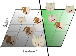
As a example, maybe we have recorded tail lengths, weights, and snout lengths from a disorganized vet clinic database that is missing some of the animals’ labels (e.g., cat vs dog). For simplicity, let’s say that this vet clinic only treats cats and dogs. With the help of neural networks, we could use a labelled dataset to learn a function mapping from tail length, weight, and snout length to the animal’s species label (i.e., a cat or a dog).
| Tail length (in) | Weight (lbs) | Snout length (in) | Label |
|---|---|---|---|
| 12.2 | 10.1 | 1.1 | cat |
| 11.6 | 9.8 | .82 | cat |
| 9.5 | 61.2 | 2.6 | dog |
| 9.1 | 65.7 | 2.9 | dog |
| … | … | … | … |
| 11.2 | 12.1 | .91 | cat |
In the above table used to train a neural network model, the model learns how best to map the observed features (tail length, weight, and snout length) to their assigned classes. After the model is trained, it can be used to infer the labels of unlabelled samples (so long as they hae tail length, weight, and snouth length recorded).
The Perceptron
The diagram above shows a perceptron — the computational unit that makes up artificial neural networks. Perceptrons are inspired by real biological neurons. From the diagram, we can see that the perceptron…
- Input features: Receives multiple input features and returns a single output
- Weights connecting features: Has adjustable weights which scale the impact of individual inputs
- Nonlinear activation function: Has a nonlinear activation function which takes as input, the weighted sum of inputs. If the sum is above some threshold, the neuron “fires” a signal (outputs -1 or 1 which represents two different class labels)
The goal then is to determine what specific weight values will allow us to separate the two classes based on the input features (e.g., shown below).

In order to determine the optimal weights, we will need to “train” the model on a labelled “training” dataset. As we pass each observation in the training data to the model, the model is able to adjust its weights in a direction that leads better performance. By training the model on many observations, we can derive weights that can accurately classify cats and dogs based on the observed input features. More explicitly, its training method can be outlined as follows:
Training algorithm
-
Initialize weights: The perceptron model starts with randomly initialized weights. These weights are the parameters/coefficients that the model will learn during training to make accurate predictions.
-
Input data: The perceptron model takes in the input data, which consists of feature vectors representing the input samples, and their corresponding labels or target values.
-
Compute weighted sum: The model computes the weighted sum of the input features by multiplying the feature values with their corresponding weights, and summing them up. This is followed by adding the bias term.
-
Activation function: The perceptron model applies an activation function, typically a step function or a threshold function, to the computed weighted sum. The activation function determines the output of the perceptron, usually producing a binary output of 0 or 1.
-
Compare with target label: The output of the perceptron is compared with the target label of the input sample to determine the prediction error. If the prediction is correct, no weight updates are made. If the prediction is incorrect, the weights and bias are updated to minimize the error.
-
Update weights: The perceptron model updates the weights based on a learning rate and the prediction error. The learning rate determines the step size of the weight updates, and it is a hyperparameter that needs to be tuned. The weights are updated using the formula:
weight_new = weight_old + learning_rate * (target - prediction) * feature
Perceptron limitations
A single perceptron cannot solve any function that is not linearly separable, meaning that we need to be able to divide the classes of inputs and outputs with a straight line. To overcome this key limitation of the perceptron (a single aritifical neuron), we need to stack together multiple perceptrons in a hierarchical fashion. Such models are referred to as multilayer perceptrons or simply neural networks
The multilayer perceptron (MLP)
To overcome the limitation of the perceptron, we can stack together multiple perceptrons in a multilayer neural network (shown below) called a multilayer perceptron (MLP). An MLP refers to a type of artificial neural network (ANN) that consists of multiple layers of interconnected nodes (neurons) organized in a feedforward manner. It typically has one or more hidden layers between the input and output layers, with each hidden layer applying an activation function to the weighted sum of its inputs. By stacking together layers of perceptrons, the MLP model can learn complex non-linear relationships in the data and make predictions based on those learned patterns.
In the diagram above, the general structure of a multilayer neural network is shown with…
- Input Layer: The input layer is the first layer of the MLP and consists of input nodes that receive the features of the input data. Each node in the input layer represents a feature or attribute of the input data. The input layer is not involved in any computation or activation; it simply passes the input features to the next layer.
- Hidden Layer(s): The hidden layers are the intermediate layers between the input and output layers. In the above diagram, there is only 1 hidden layer, but MLPs often have more. They are called “hidden” because their outputs are not directly visible in the input or output data. Each hidden layer consists of multiple nodes (neurons) that compute a weighted sum of the inputs from the previous layer, followed by an activation function. The number of hidden layers and the number of nodes in each hidden layer are hyperparameters that can be tuned during model design and training.
- Weighted Connections: Each connection between nodes in adjacent layers has a weight associated with it. These weights are the parameters that the model learns during training to determine the strength of the connections. The weighted sum of inputs to a node is computed by multiplying the input values with their corresponding weights and summing them up. Also referred to as “weights” for short.
- Weights: The weights of each neuron send its (weighted) output to each neuron in the subsequent layer
- Output Layer: The output layer is the last layer of the MLP and produces the final output of the model. It typically consists of one or more nodes, depending on the specific task. For binary classification, a single output node with a sigmoid activation function is commonly used. For multi-class classification, multiple output nodes with a softmax activation function are used. For regression tasks, a single output node with a linear activation function is often used.
Training algorithm
Similar to the perceptron, the MLP is trained using a supervised learning algorithm that updates the weights iteratively based on the prediction error of each training sample.
- Initialization: The network’s weights are randomly initialized.
- Forward Propagation: Input data is fed through the network from input nodes to output nodes, with weights applied at each connection, and the output is computed.
- Error Calculation: The difference between the predicted output and the actual output (target) is calculated as the error.
- Backpropagation: The error is propagated backward through the network, and the weights are adjusted to minimize the error.
- Iterative Process: Steps 2-4 are repeated for multiple iterations or epochs, with input data fed through the network and weights updated until the network’s performance converges to a satisfactory level.
- Function Mapping: Once the network is trained, it can be used to map new input data to corresponding outputs, leveraging the learned weights.
Deriving New Features from Neural Networks
After training a neural network, the neural weights encode new features of the data that are conducive to performing well on whatever task the neural network is given. This is due to the feedforward processing built into the network — the outputs of previous layers are sent to subsequent layers, and the so additional transformations get applied to the original inputs as they transcend the network.
Generally speaking, the deeper the neural network is, the more complicated/abstract these features can become. We call this a hierarchical feature representation. For example, in deep convolutional neural networks (a special kind of neural network designed for image processing), the features in each layer look something like the image shown below when the model is trained on a facial recognition task.

Training Word2Vec to Learn Word Embeddings
Recall that the ultimate goal of the Word2Vec method is to output meaningful word embeddings/vectors. How can we train a neural network for such a task? We could try to tediously hand-craft a large list of word vectors that have the properties we seek (e.g., similar words have similar vectors), and then train a neural network to learn this mapping before applying it to new words. However, crafting a list of vectors manually would be an arudous task. Furthermore, it is not immediately clear what kind of vector representation would be best.
Instead, we can capitalize on the fact that neural networks are well posed to learn new features from the input data. Specifically, the new features will be features that are useful for whatever task the model is assigned. With this consideration, we can devise a language related task that allows a neural network model to learn interesting features of words which can then be extracted from the model as a word embedding representation (i.e., a vector). We’ll unpack how the embedding gets extracted from the trained model shortly. For now, let’s focus on what kind of language-related task to give the model.
Predicting context words
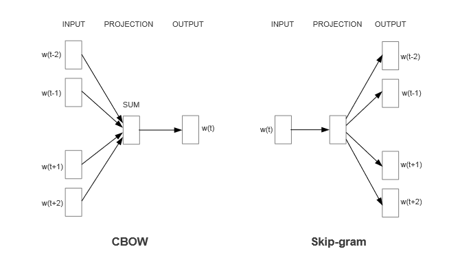
What task can we give a neural network to learn meaningful word embeddings? Our friend RJ Firth gives us a hint when he says, “You shall know a word by the company it keeps.” Using the distributional hypothesis as motivation, which states that words that repeatedly occur in similar contexts probably have similar meanings, we can ask a neural network to predict the context words that surround a given word in a sentence. The Skip-gram algorithm shown on the right side of the below diagram does just that.

Sentence Processing With Skip-Gram
The Skip-gram version takes as input each word in a sentence, and tries to guess the most likely surrounding context words associated with that word. It does this for all sentences and words in a corpus in order to learn a function that can map each word to its most likely context words.
Have a very nice day.
| Input | Output (context words) |
|---|---|
| Have | a, very |
| a | Have, very, nice |
| very | Have, a, nice, day |
| nice | a, very, day |
| day | very, nice |
In the process of training, the model’s weights learn to derive new features (weight optimized perceptrons) associated with the input data (single words). These new learned features will be conducive to accurately predicting the context words for each word. We will see next how we can extract these features as word vectors.
Extracting Word Embeddings From the Model
With a model trained to predict context words, how can we extract the model’s learned features as word embeddings? For this, we need a set of model weights associated with each word fed into the model. We can achieve this property by:
- Converting each input word into a one-hot encoded vector representation. The vector dimensionality will be equal to the size of the vocabularly contained in the training data.
- Connecting each element of the one-hot encoded vector to each node/neuron in the subsequent hidden layer of neurons
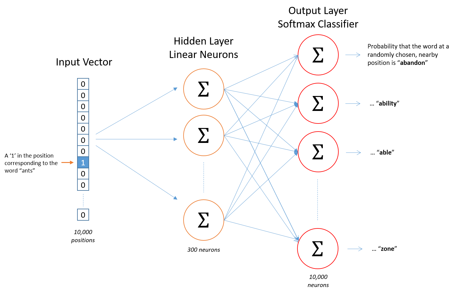
These steps can be visualized in the Word2Vec model diagram shown below, with Sigmas representing individual neurons and their ability to integrate input from previous layers.

In the above digram, we can see…
- The input layer has 10,000 dimensions representing 10,000 words in this model’s vocabulary
- The hidden layer of the model has 300 neurons. Note that this number also corresponds to the dimensionality of the word vectors extracted from the model.
- The output layer has one neuron for each possible word in the model’s vocabulary
The word vectors, themselves, are stored in the weights connecting the input layer to the hidden layer of neurons. Each word will have its own set of learned weights which we call word vectors. You can think of each element of the word vectors as encoding different features which are relevant to the prediction task at hand — predicting context words.
Continuous Bag-of-Words (CBOW)

Before wrapping up with the mechanisms underlying the Word2Vec model, it is important to mention that the Skip-gram algorithm is not the only way to train word embeddings using Word2Vec. A similar method known as the Continuous Bag-of-Words (CBOW) takes as an input the context words surrounding a target word, and tries to guess the target word based on those words. Thus, it flips the prediction task faced by Skip-gram. The CBOW algorithm does not care how far away different context words are from the target word, which is why it is called a bag-of-words method. With this task setup, the neural network will learn a function that can map the surrounding context words to a target word. Similar to Skip-gram, the CBOW method will generate word vectors stored as weights of the neural network. However, given the slight adjustment in task, the weights extracted from CBOW are the ones that connect the hidden layer of neurons to the output layer.
CBOW vs Skip-gram
Since there are two popular word2vec training methods, how should we decide which one to pick? Like with many things in machine learning, the best course of action is typically to take a data-driven approach to see which one works better for your specific application. However, as general guidelines according to Mikolov et al.,
- Skip-Gram works well with smaller datasets and has been found to perform better in terms of its ability to represent rarer words
- CBOW trains several times faster than Skip-gram and has slightly better accuracy for more frequent words
Recap
Artificial neural networks are powerful machine learning models that can learn to map input data containing features to a predicted label or continuous value. In addition, neural networks learn to encode the input data as hierarchical features of the text during training. The Word2Vec model exploits this capability, and trains the model on a word prediction task in order to generate features of words which are conducive to the prediction task at hand.
In the next episode, we’ll train a Word2Vec model using both training methods and empirically evaluate the performance of each. We’ll also see how training Word2Vec models from scratch (rather than using a pretrained model) can be beneficial in some circumstances.
Key Points
Artificial neural networks (ANNs) are powerful models that can approximate any function given sufficient training data.
The best method to decide between training methods (CBOW and Skip-gram) is to try both methods and see which one works best for your specific application.

