Python Fundamentals

Overview

Teaching: 20 min
Exercises: 10 min

Questions

• What basic data types can I work with in Python?

• How can I create a new variable in Python?

• How do I use a function?

• Can I change the value associated with a variable after I create it?

Objectives

• Assign values to variables.

Variables

Any Python interpreter can be used as a calculator:

3 + 5 * 4

23

This is great but not very interesting. To do anything useful with data, we need to assign its value to a variable. In Python, we can assign a value to a variable, using the equals sign =. For example we can capture the gross domestic power per capita for a country by assinging the value ? to a variable gdpPercapUSD:

gdpPercapUSD = 2449

From now on, whenever we use gdpPercapUSD, Python will substitute the value we assigned to it. In layman’s terms, a variable is a name for a value.

In Python, variable names:

• can include letters, digits, and underscores
• cannot start with a digit
• are case sensitive.

This means that, for example:

• gdpPercap0 is a valid variable name, whereas 0gdpPercap is not
• gdp_percap and GDP_percap are different variables

Types of data

Python knows various types of data. Three common ones are:

• integer numbers
• floating point numbers, and
• strings.

In the example above, variable gdpPercapUSD has an integer value of 2449. If we want to capture the gdp per capita of the country more precisely we can use a floating point value by executing:

gdpPercapUSD = 2449.008185

To create a string, we add single or double quotes around some text. To keep track of the year we are working with we can store the year in a string:

year = "1952"

Using Variables in Python

Once we have data stored with variable names, we can make use of it in calculations. We may want to store the country’s gdp percapita in US dollars and in British pounds:

gdpPercapGBP = gdpPercapUSD * 0.779063

We could add the year to the label gdpPercap_

columnlabel = 'gdpPercap_' + year

Built-in Python functions

To carry out common tasks with data and variables in Python, the language provides us with several built-in functions. To display information to the screen, we use the print function:

print(gdpPercapUSD)
print(gdpPercapGBP)
print(columnlabel)

2249.008185
1752.119063630655
gdpPercap_1952

When we want to make use of a function, referred to as calling the function, we follow its name by parentheses. The parentheses are important: if you leave them off, the function doesn’t actually run! Sometimes you will include values or variables inside the parentheses for the function to use. In the case of print, we use the parentheses to tell the function what value we want to display. We will learn more about how functions work and how to create our own in later episodes.

We can display multiple things at once using only one print call:

print(columnlabel , 'for Algeria:' , gdpPercapUSD , '(USD)')

gdpPercap_1952 for Algeria: 2249.008185 (USD)

We can also call a function inside of another function call. For example, Python has a built-in function called type that tells you a value’s data type:

print(type(2249.008185))
print(type(columnlabel))

<class 'float'>
<class 'str'>

Moreover, we can do arithmetic with variables right inside the print function:

print('gdpPercap in GBP:', gdpPercapUSD * 0.779063)

gdpPercap in GBP: 1752.119063630655

The above command, however, did not change the value of gdpPercapUSD:

print(gdpPercapUSD)

2249.008185

To change the value of the gdpPercapUSD variable, we have to assign gdpPercapUSD a new value using the equals = sign:

gdpPercapUSD = 3520.610273	
print('The gdp per capita for Angola in USD is:', gdpPercapUSD)

The gdp per capita for Angola in USD is: 3520.610273

Variables as Sticky Notes

A variable in Python is analogous to a sticky note with a name written on it: assigning a value to a variable is like putting that sticky note on a particular value.

Using this analogy, we can investigate how assigning a value to one variable does not change values of other, seemingly related, variables. For example, let’s store the, country Angola’s, gdp per capita GPB in its own variable:

# gdp per capita for Angola
gdpPercapGBP = gdpPercapUSD * 0.779090
print('gdp per capita in GBP', gdpPercapGBP, 'and in USD:', gdpPercapUSD)

gdp per capita in GBP 2742.8722575915695 and in USD: 3520.610273

Similar to above, the expression gdpPercapUSD * 0.779090 is evaluated to 2742.8722575915695, and then this value is assigned to the variable gdpPercapGBP (i.e. the sticky note gdpPercapGBP is placed on 2742.8722575915695). At this point, each variable is “stuck” to completely distinct and unrelated values.

Let’s now change gdpPercapUSD:

gdpPercapUSD = 851.241141
print('gdp percapita in USD is now:', gdpPercapUSD, 'and gdp per capita in GBP is still: ', gdpPercapGBP)

gdp percapita in USD is now: 851.241141 and gdp per capita in GBP is still:  2742.8722575915695

Since gdpPercapGBP doesn’t “remember” where its value comes from, it is not updated when we change gdpPercapUSD.

Check Your Understanding

What values do the variables mass and age have after each of the following statements? Test your answer by executing the lines.

mass = 47.5
age = 122
mass = mass * 2.0
age = age - 20

Solution

`mass` holds a value of 47.5, `age` does not exist
`mass` still holds a value of 47.5, `age` holds a value of 122
`mass` now has a value of 95.0, `age`'s value is still 122
`mass` still has a value of 95.0, `age` now holds 102

Sorting Out References

Python allows you to assign multiple values to multiple variables in one line by separating the variables and values with commas. What does the following program print out?

first, second = 'Grace', 'Hopper'
third, fourth = second, first
print(third, fourth)

Solution

Hopper Grace

Seeing Data Types

What are the data types of the following variables?

planet = 'Earth'
apples = 5
distance = 10.5

Solution

type(planet)
type(apples)
type(distance)

<class 'str'>
<class 'int'>
<class 'float'>

Key Points

• Basic data types in Python include integers, strings, and floating-point numbers.

• Use variable = value to assign a value to a variable in order to record it in memory.

• Variables are created on demand whenever a value is assigned to them.

• Use print(something) to display the value of something.

• Built-in functions are always available to use.

Analyzing Data

Overview

Teaching: 40 min
Exercises: 20 min

Questions

• What dataset are we using today?

• How can I process tabular data files in Python?

Objectives

• Introduce dataset

• Explain what a library is and what libraries are used for.

• Import the Pandas library

• Use Pandas to read a simple CSV data set

• Get some basic information about a Pandas Dataframe

Our dataset

We are using a dataset generated by Gapminder which describes income per person (GDP per capita) and life expectancy over a series of years between 1952 and 2007. We have a csv file for each continent and another that combines all data.

The data sets are stored in comma-separated values (CSV) format with each row holding information on a single country.

The first three rows of the first file look like this:

"continent","country","gdpPercap_1952","gdpPercap_1957","gdpPercap_1962","gdpPercap_1967","gdpPercap_1972","gdpPercap_1977","gdpPercap_1982","gdpPercap_1987","gdpPercap_1992","gdpPercap_1997","gdpPercap_2002","gdpPercap_2007","lifeExp_1952","lifeExp_1957","lifeExp_1962","lifeExp_1967","lifeExp_1972","lifeExp_1977","lifeExp_1982","lifeExp_1987","lifeExp_1992","lifeExp_1997","lifeExp_2002","lifeExp_2007","pop_1952","pop_1957","pop_1962","pop_1967","pop_1972","pop_1977","pop_1982","pop_1987","pop_1992","pop_1997","pop_2002","pop_2007"
"Africa","Algeria",2449.008185,3013.976023,2550.81688,3246.991771,4182.663766,4910.416756,5745.160213,5681.358539,5023.216647,4797.295051,5288.040382,6223.367465,43.077,45.685,48.303,51.407,54.518,58.014,61.368,65.799,67.744,69.152,70.994,72.301,9279525,10270856,11000948,12760499,14760787,17152804,20033753,23254956,26298373,29072015,31287142,33333216
"Africa","Angola",3520.610273,3827.940465,4269.276742,5522.776375,5473.288005,3008.647355,2756.953672,2430.208311,2627.845685,2277.140884,2773.287312,4797.231267,30.015,31.999,34,35.985,37.928,39.483,39.942,39.906,40.647,40.963,41.003,42.731,4232095,4561361,4826015,5247469,5894858,6162675,7016384,7874230,8735988,9875024,10866106,12420476

We’ll learn more about how programming can help us explore this data.

Libraries

Words are useful, but what’s more useful are the sentences and stories we build with them. Similarly, while a lot of powerful, general tools are built into Python, specialized tools built up from these basic units live in libraries that can be called upon when needed.

Use the Pandas library to do explore tabular data.

Importing a library is like getting a piece of lab equipment out of a storage locker and setting it up on the bench. Libraries provide additional functionality to the basic Python package, much like a new piece of equipment adds functionality to a lab space. Just like in the lab, importing too many libraries can sometimes complicate and slow down your programs - so we only import what we need for each program.

• Pandas is a widely-used Python library for statistics, particularly on tabular data.
• Borrows many features from R’s dataframes.
  • A 2-dimensional table whose columns have names and potentially have different data types.
• Load it with import pandas as pd. The alias pd is commonly used for Pandas.
• Read a Comma Separated Values (CSV) data file with pd.read_csv.
  • Argument is the name of the file to be read.
  • Assign result to a variable to store the data that was read.

Once we’ve imported the library, we can ask the library to read our data file for us:

import pandas as pd

data = pd.read_csv('data/gapminder_gdp_oceania.csv')
print(data)

       country  gdpPercap_1952  gdpPercap_1957  gdpPercap_1962  \
0    Australia     10039.59564     10949.64959     12217.22686
1  New Zealand     10556.57566     12247.39532     13175.67800

   gdpPercap_1967  gdpPercap_1972  gdpPercap_1977  gdpPercap_1982  \
0     14526.12465     16788.62948     18334.19751     19477.00928
1     14463.91893     16046.03728     16233.71770     17632.41040

   gdpPercap_1987  gdpPercap_1992  gdpPercap_1997  gdpPercap_2002  \
0     21888.88903     23424.76683     26997.93657     30687.75473
1     19007.19129     18363.32494     21050.41377     23189.80135

   gdpPercap_2007
0     34435.36744
1     25185.00911

The expression pd.read_csv is a function call that asks Python to run the function read_csv which belongs to the pandas library. This dotted notation is used everywhere in Python: the thing that appears before the dot contains the thing that appears after.

As an example, John Smith is the John that belongs to the Smith family. We could use the dot notation to write his name smith.john, just as read_csv is a function that belongs to the pandas library.

pandas.read_csv has one parameter: the name of the file we want to read. This needs to be character string (or string for short), so we put it in quotes.

Our call read our file and saved the data in memory to a variable called data. We then checked our data had been loaded successfully by printing the variable’s value to the screen.

Pandas uses backslash \ to show wrapped lines when output is too wide to fit the screen.

File Not Found

Our lessons store their data files in a data sub-directory, which is why the path to the file is data/gapminder_gdp_oceania.csv. If you forget to include data/, or if you include it but your copy of the file is somewhere else, you will get a runtime error that ends with a line like this:

FileNotFoundError: [Errno 2] No such file or directory: 'data/gapminder_gdp_oceania.csv'

Now that the data are in memory, we can manipulate them.

Use index_col to specify that a column’s values should be used as row headings.

• Row headings are numbers (0 and 1 in this case).
• Really want to index by country.
• Pass the name of the column to read_csv as its index_col parameter to do this.

data = pd.read_csv('data/gapminder_gdp_oceania.csv', index_col='country')
print(data)

             gdpPercap_1952  gdpPercap_1957  gdpPercap_1962  gdpPercap_1967  \
country
Australia       10039.59564     10949.64959     12217.22686     14526.12465
New Zealand     10556.57566     12247.39532     13175.67800     14463.91893

             gdpPercap_1972  gdpPercap_1977  gdpPercap_1982  gdpPercap_1987  \
country
Australia       16788.62948     18334.19751     19477.00928     21888.88903
New Zealand     16046.03728     16233.71770     17632.41040     19007.19129

             gdpPercap_1992  gdpPercap_1997  gdpPercap_2002  gdpPercap_2007
country
Australia       23424.76683     26997.93657     30687.75473     34435.36744
New Zealand     18363.32494     21050.41377     23189.80135     25185.00911

Use the DataFrame.info() method to find out more about a dataframe.

data.info()

<class 'pandas.core.frame.DataFrame'>
Index: 2 entries, Australia to New Zealand
Data columns (total 12 columns):
gdpPercap_1952    2 non-null float64
gdpPercap_1957    2 non-null float64
gdpPercap_1962    2 non-null float64
gdpPercap_1967    2 non-null float64
gdpPercap_1972    2 non-null float64
gdpPercap_1977    2 non-null float64
gdpPercap_1982    2 non-null float64
gdpPercap_1987    2 non-null float64
gdpPercap_1992    2 non-null float64
gdpPercap_1997    2 non-null float64
gdpPercap_2002    2 non-null float64
gdpPercap_2007    2 non-null float64
dtypes: float64(12)
memory usage: 208.0+ bytes

• This is a DataFrame
• Two rows named 'Australia' and 'New Zealand'
• Twelve columns, each of which has two actual 64-bit floating point values.
  • We will talk later about null values, which are used to represent missing observations.
• Uses 208 bytes of memory.

The DataFrame.columns variable stores information about the dataframe’s columns.

• Note that this is data, not a method. (It doesn’t have parentheses.)
  • Like math.pi.
  • So do not use () to try to call it.
• Called a member variable, or just member.

print(data.columns)

Index(['gdpPercap_1952', 'gdpPercap_1957', 'gdpPercap_1962', 'gdpPercap_1967',
       'gdpPercap_1972', 'gdpPercap_1977', 'gdpPercap_1982', 'gdpPercap_1987',
       'gdpPercap_1992', 'gdpPercap_1997', 'gdpPercap_2002', 'gdpPercap_2007'],
      dtype='object')

Use DataFrame.T to transpose a dataframe.

• Sometimes want to treat columns as rows and vice versa.
• Transpose (written .T) doesn’t copy the data, just changes the program’s view of it.
• Like columns, it is a member variable.
• We will use this again when we try and plot the data.

print(data.T)

country           Australia  New Zealand
gdpPercap_1952  10039.59564  10556.57566
gdpPercap_1957  10949.64959  12247.39532
gdpPercap_1962  12217.22686  13175.67800
gdpPercap_1967  14526.12465  14463.91893
gdpPercap_1972  16788.62948  16046.03728
gdpPercap_1977  18334.19751  16233.71770
gdpPercap_1982  19477.00928  17632.41040
gdpPercap_1987  21888.88903  19007.19129
gdpPercap_1992  23424.76683  18363.32494
gdpPercap_1997  26997.93657  21050.41377
gdpPercap_2002  30687.75473  23189.80135
gdpPercap_2007  34435.36744  25185.00911

Note about Pandas DataFrames/Series

A DataFrame is a collection of Series; The DataFrame is the way Pandas represents a table, and Series is the data-structure Pandas use to represent a column.

Pandas is built on top of the Numpy library, which in practice means that most of the methods defined for Numpy Arrays apply to Pandas Series/DataFrames.

What makes Pandas so attractive is the powerful interface to access individual records of the table, proper handling of missing values, and relational-databases operations between DataFrames.

Selecting values

To access a value at the position [i,j] of a DataFrame, we have two options, depending on what is the meaning of i in use. Remember that a DataFrame provides an index as a way to identify the rows of the table; a row, then, has a position inside the table as well as a label, which uniquely identifies its entry in the DataFrame.

Use DataFrame.iloc[..., ...] to select values by their (entry) position

• Can specify location by numerical index analogously to 2D version of character selection in strings.

import pandas as pd
data = pd.read_csv('data/gapminder_gdp_europe.csv', index_col='country')
print(data.iloc[0, 0])

1601.056136

The expression data[30, 20] accesses the element at row 30, column 20. While this expression may not surprise you, data[0, 0] might. Programming languages like Fortran, MATLAB and R start counting at 1 because that’s what human beings have done for thousands of years. Languages in the C family (including C++, Java, Perl, and Python) count from 0 because it represents an offset from the first value in the array (the second value is offset by one index from the first value). This is closer to the way that computers represent arrays (if you are interested in the historical reasons behind counting indices from zero, you can read Mike Hoye’s blog post). As a result, if we have an M×N array in Python, its indices go from 0 to M-1 on the first axis and 0 to N-1 on the second. It takes a bit of getting used to, but one way to remember the rule is that the index is how many steps we have to take from the start to get the item we want.

In the Corner

What may also surprise you is that when Python displays an array, it shows the element with index [0, 0] in the upper left corner rather than the lower left. This is consistent with the way mathematicians draw matrices but different from the Cartesian coordinates. The indices are (row, column) instead of (column, row) for the same reason, which can be confusing when plotting data.

Use DataFrame.loc[..., ...] to select values by their (entry) label.

• Can specify location by row name analogously to 2D version of dictionary keys.

print(data.loc["Albania", "gdpPercap_1952"])

1601.056136

Use : on its own to mean all columns or all rows.

• Just like Python’s usual slicing notation.

print(data.loc["Albania", :])

gdpPercap_1952    1601.056136
gdpPercap_1957    1942.284244
gdpPercap_1962    2312.888958
gdpPercap_1967    2760.196931
gdpPercap_1972    3313.422188
gdpPercap_1977    3533.003910
gdpPercap_1982    3630.880722
gdpPercap_1987    3738.932735
gdpPercap_1992    2497.437901
gdpPercap_1997    3193.054604
gdpPercap_2002    4604.211737
gdpPercap_2007    5937.029526
Name: Albania, dtype: float64

• Would get the same result printing data.loc["Albania"] (without a second index).

print(data.loc[:, "gdpPercap_1952"])

country
Albania                    1601.056136
Austria                    6137.076492
Belgium                    8343.105127
⋮ ⋮ ⋮
Switzerland               14734.232750
Turkey                     1969.100980
United Kingdom             9979.508487
Name: gdpPercap_1952, dtype: float64

• Would get the same result printing data["gdpPercap_1952"]
• Also get the same result printing data.gdpPercap_1952 (not recommended, because easily confused with . notation for methods)

Select multiple columns or rows using DataFrame.loc and a named slice.

print(data.loc['Italy':'Poland', 'gdpPercap_1962':'gdpPercap_1972'])

             gdpPercap_1962  gdpPercap_1967  gdpPercap_1972
country
Italy           8243.582340    10022.401310    12269.273780
Montenegro      4649.593785     5907.850937     7778.414017
Netherlands    12790.849560    15363.251360    18794.745670
Norway         13450.401510    16361.876470    18965.055510
Poland          5338.752143     6557.152776     8006.506993

In the above code, we discover that slicing using loc is inclusive at both ends, which differs from slicing using iloc, where slicing indicates everything up to but not including the final index.

Result of slicing can be used in further operations.

• Usually don’t just print a slice.
• All the statistical operators that work on entire dataframes work the same way on slices.
• E.g., calculate max of a slice.

print(data.loc['Italy':'Poland', 'gdpPercap_1962':'gdpPercap_1972'].max())

gdpPercap_1962    13450.40151
gdpPercap_1967    16361.87647
gdpPercap_1972    18965.05551
dtype: float64

print(data.loc['Italy':'Poland', 'gdpPercap_1962':'gdpPercap_1972'].min())

gdpPercap_1962    4649.593785
gdpPercap_1967    5907.850937
gdpPercap_1972    7778.414017
dtype: float64

Not All Functions Have Input

Generally, a function uses inputs to produce outputs. However, some functions produce outputs without needing any input. For example, checking the current time doesn’t require any input.

import time
print(time.ctime())

Sat Mar 26 13:07:33 2016

For functions that don’t take in any arguments, we still need parentheses (()) to tell Python to go and do something for us.

Slicing Strings

A section of an array is called a slice. We can take slices of character strings as well:

element = 'oxygen'
print('first three characters:', element[0:3])
print('last three characters:', element[3:6])

first three characters: oxy
last three characters: gen

What is the value of element[:4]? What about element[4:]? Or element[:]?

Solution

oxyg
en
oxygen

What is element[-1]? What is element[-2]?

Solution

n
e

Given those answers, explain what element[1:-1] does.

Solution

Creates a substring from index 1 up to (not including) the final index, effectively removing the first and last letters from ‘oxygen’

How can we rewrite the slice for getting the last three characters of element, so that it works even if we assign a different string to element? Test your solution with the following strings: carpentry, clone, hi.

Solution

element = 'oxygen'
print('last three characters:', element[-3:])
element = 'carpentry'
print('last three characters:', element[-3:])
element = 'clone'
print('last three characters:', element[-3:])
element = 'hi'
print('last three characters:', element[-3:])

last three characters: gen
last three characters: try
last three characters: one
last three characters: hi

Selection of Individual Values

Assume Pandas has been imported into your notebook and the Gapminder GDP data for Europe has been loaded:

import pandas as pd

df = pd.read_csv('data/gapminder_gdp_europe.csv', index_col='country')

Write an expression to find the Per Capita GDP of Serbia in 2007.

Solution

The selection can be done by using the labels for both the row (“Serbia”) and the column (“gdpPercap_2007”):

print(df.loc['Serbia', 'gdpPercap_2007'])

The output is

9786.534714

Extent of Slicing

1. Do the two statements below produce the same output?
2. Based on this, what rule governs what is included (or not) in numerical slices and named slices in Pandas?

print(df.iloc[0:2, 0:2])
print(df.loc['Albania':'Belgium', 'gdpPercap_1952':'gdpPercap_1962'])

Solution

No, they do not produce the same output! The output of the first statement is:

        gdpPercap_1952  gdpPercap_1957
country                                
Albania     1601.056136     1942.284244
Austria     6137.076492     8842.598030

The second statement gives:

        gdpPercap_1952  gdpPercap_1957  gdpPercap_1962
country                                                
Albania     1601.056136     1942.284244     2312.888958
Austria     6137.076492     8842.598030    10750.721110
Belgium     8343.105127     9714.960623    10991.206760

Clearly, the second statement produces an additional column and an additional row compared to the first statement.
What conclusion can we draw? We see that a numerical slice, 0:2, omits the final index (i.e. index 2) in the range provided, while a named slice, ‘gdpPercap_1952’:’gdpPercap_1962’, includes the final element.

Reconstructing Data

Explain what each line in the following short program does: what is in first, second, etc.?

first = pd.read_csv('data/gapminder_all.csv', index_col='country')
second = first[first['continent'] == 'Americas']
third = second.drop('Puerto Rico')
fourth = third.drop('continent', axis = 1)
fourth.to_csv('result.csv')

Solution

Let’s go through this piece of code line by line.

first = pd.read_csv('data/gapminder_all.csv', index_col='country')

This line loads the dataset containing the GDP data from all countries into a dataframe called first. The index_col='country' parameter selects which column to use as the row labels in the dataframe.

second = first[first['continent'] == 'Americas']

This line makes a selection: only those rows of first for which the ‘continent’ column matches ‘Americas’ are extracted. Notice how the Boolean expression inside the brackets, first['continent'] == 'Americas', is used to select only those rows where the expression is true. Try printing this expression! Can you print also its individual True/False elements? (hint: first assign the expression to a variable)

third = second.drop('Puerto Rico')

As the syntax suggests, this line drops the row from second where the label is ‘Puerto Rico’. The resulting dataframe third has one row less than the original dataframe second.

fourth = third.drop('continent', axis = 1)

Again we apply the drop function, but in this case we are dropping not a row but a whole column. To accomplish this, we need to specify also the axis parameter (we want to drop the second column which has index 1).

fourth.to_csv('result.csv')

The final step is to write the data that we have been working on to a csv file. Pandas makes this easy with the to_csv() function. The only required argument to the function is the filename. Note that the file will be written in the directory from which you started the Jupyter or Python session.

Selecting Indices

Explain in simple terms what idxmin and idxmax do in the short program below. When would you use these methods?

data = pd.read_csv('data/gapminder_gdp_europe.csv', index_col='country')
print(data.idxmin())
print(data.idxmax())

Solution

For each column in data, idxmin will return the index value corresponding to each column’s minimum; idxmax will do accordingly the same for each column’s maximum value.

You can use these functions whenever you want to get the row index of the minimum/maximum value and not the actual minimum/maximum value.

Practice with Selection

Assume Pandas has been imported and the Gapminder GDP data for Europe has been loaded. Write an expression to select each of the following:

1. GDP per capita for all countries in 1982.
2. GDP per capita for Denmark for all years.
3. GDP per capita for all countries for years after 1985.
4. GDP per capita for each country in 2007 as a multiple of GDP per capita for that country in 1952.

Solution

1:

data['gdpPercap_1982']

2:

data.loc['Denmark',:]

3:

data.loc[:,'gdpPercap_1985':]

Pandas is smart enough to recognize the number at the end of the column label and does not give you an error, although no column named gdpPercap_1985 actually exists. This is useful if new columns are added to the CSV file later.

4:

data['gdpPercap_2007']/data['gdpPercap_1952']

Many Ways of Access

There are at least two ways of accessing a value or slice of a DataFrame: by name or index. However, there are many others. For example, a single column or row can be accessed either as a DataFrame or a Series object.

Suggest different ways of doing the following operations on a DataFrame:

1. Access a single column
2. Access a single row
3. Access an individual DataFrame element
4. Access several columns
5. Access several rows
6. Access a subset of specific rows and columns
7. Access a subset of row and column ranges

Solution

1. Access a single column:

# by name
data["col_name"]   # as a Series
data[["col_name"]] # as a DataFrame

# by name using .loc
data.T.loc["col_name"]  # as a Series
data.T.loc[["col_name"]].T  # as a DataFrame

# Dot notation (Series)
data.col_name

# by index (iloc)
data.iloc[:, col_index]   # as a Series
data.iloc[:, [col_index]] # as a DataFrame

# using a mask
data.T[data.T.index == "col_name"].T

2. Access a single row:

# by name using .loc
data.loc["row_name"] # as a Series
data.loc[["row_name"]] # as a DataFrame

# by name
data.T["row_name"] # as a Series
data.T[["row_name"]].T as a DataFrame

# by index
data.iloc[row_index]   # as a Series
data.iloc[[row_index]]   # as a DataFrame

# using mask
data[data.index == "row_name"]

3. Access an individual DataFrame element:

# by column/row names
data["column_name"]["row_name"]         # as a Series

data[["col_name"]].loc["row_name"]  # as a Series
data[["col_name"]].loc[["row_name"]]  # as a DataFrame

data.loc["row_name"]["col_name"]  # as a value
data.loc[["row_name"]]["col_name"]  # as a Series
data.loc[["row_name"]][["col_name"]]  # as a DataFrame

data.loc["row_name", "col_name"]  # as a value
data.loc[["row_name"], "col_name"]  # as a Series. Preserves index. Column name is moved to `.name`.
data.loc["row_name", ["col_name"]]  # as a Series. Index is moved to `.name.` Sets index to column name.
data.loc[["row_name"], ["col_name"]]  # as a DataFrame (preserves original index and column name)

# by column/row names: Dot notation
data.col_name.row_name

# by column/row indices
data.iloc[row_index, col_index] # as a value
data.iloc[[row_index], col_index] # as a Series. Preserves index. Column name is moved to `.name`
data.iloc[row_index, [col_index]] # as a Series. Index is moved to `.name.` Sets index to column name.
data.iloc[[row_index], [col_index]] # as a DataFrame (preserves original index and column name)

# column name + row index
data["col_name"][row_index]
data.col_name[row_index]
data["col_name"].iloc[row_index]

# column index + row name
data.iloc[:, [col_index]].loc["row_name"]  # as a Series
data.iloc[:, [col_index]].loc[["row_name"]]  # as a DataFrame

# using masks
data[data.index == "row_name"].T[data.T.index == "col_name"].T

4. Access several columns:

# by name
data[["col1", "col2", "col3"]]
data.loc[:, ["col1", "col2", "col3"]]

# by index
data.iloc[:, [col1_index, col2_index, col3_index]]

5. Access several rows

# by name
data.loc[["row1", "row2", "row3"]]

# by index
data.iloc[[row1_index, row2_index, row3_index]]

6. Access a subset of specific rows and columns

# by names
data.loc[["row1", "row2", "row3"], ["col1", "col2", "col3"]]

# by indices
data.iloc[[row1_index, row2_index, row3_index], [col1_index, col2_index, col3_index]]

# column names + row indices
data[["col1", "col2", "col3"]].iloc[[row1_index, row2_index, row3_index]]

# column indices + row names
data.iloc[:, [col1_index, col2_index, col3_index]].loc[["row1", "row2", "row3"]]

7. Access a subset of row and column ranges

# by name
data.loc["row1":"row2", "col1":"col2"]

# by index
data.iloc[row1_index:row2_index, col1_index:col2_index]

# column names + row indices
data.loc[:, "col1_name":"col2_name"].iloc[row1_index:row2_index]

# column indices + row names
data.iloc[:, col1_index:col2_index].loc["row1":"row2"]

Key Points

• Import a library into a program using import libraryname.

• Use the pandas library to work with arrays in Python.

• Array indices start at 0, not 1.

• Use DataFrame.iloc[..., ...] to select values by integer location.

• Use : on its own to mean all columns or all rows.

• Select multiple columns or rows using DataFrame.loc and a named slice.

• Result of slicing can be used in further operations.

Visualizing Data

Overview

Teaching: 15 min
Exercises: 15 min

Questions

• How can I plot my data?

• How can I save my plot for publishing?

Objectives

• Create a time series plot showing a single data set.

• Create a scatter plot showing relationship between two data sets.

matplotlib is the most widely used scientific plotting library in Python.

• Commonly use a sub-library called matplotlib.pyplot.
• The Jupyter Notebook will render plots inline by default.

import matplotlib.pyplot as plt

• Simple plots are then (fairly) simple to create.

time = [0, 1, 2, 3]
position = [0, 100, 200, 300]

plt.plot(time, position)
plt.xlabel('Time (hr)')
plt.ylabel('Position (km)')

Display All Open Figures

In our Jupyter Notebook example, running the cell should generate the figure directly below the code. The figure is also included in the Notebook document for future viewing. However, other Python environments like an interactive Python session started from a terminal or a Python script executed via the command line require an additional command to display the figure.

Instruct matplotlib to show a figure:

plt.show()

This command can also be used within a Notebook - for instance, to display multiple figures if several are created by a single cell.

Plot data directly from a Pandas dataframe.

• We can also plot Pandas dataframes.
• This implicitly uses matplotlib.pyplot.
• Before plotting, we convert the column headings from a string to integer data type, since they represent numerical values

import pandas as pd

data = pd.read_csv('data/gapminder_gdp_oceania.csv', index_col='country')

# Extract year from last 4 characters of each column name
# The current column names are structured as 'gdpPercap_(year)', 
# so we want to keep the (year) part only for clarity when plotting GDP vs. years
# To do this we use strip(), which removes from the string the characters stated in the argument
# This method works on strings, so we call str before strip()

years = data.columns.str.strip('gdpPercap_')

# Convert year values to integers, saving results back to dataframe

data.columns = years.astype(int)

data.loc['Australia'].plot()

Select and transform data, then plot it.

• By default, DataFrame.plot plots with the rows as the X axis.
• We can transpose the data in order to plot multiple series.

data.T.plot()
plt.ylabel('GDP per capita')

Many styles of plot are available.

• For example, do a bar plot using a fancier style.

plt.style.use('ggplot')
data.T.plot(kind='bar')
plt.ylabel('GDP per capita')

Data can also be plotted by calling the matplotlib plot function directly.

• The command is plt.plot(x, y)
• The color and format of markers can also be specified as an additional optional argument e.g., b- is a blue line, g-- is a green dashed line.

Get Australia data from dataframe

years = data.columns
gdp_australia = data.loc['Australia']

plt.plot(years, gdp_australia, 'g--')

Can plot many sets of data together.

# Select two countries' worth of data.
gdp_australia = data.loc['Australia']
gdp_nz = data.loc['New Zealand']

# Plot with differently-colored markers.
plt.plot(years, gdp_australia, 'b-', label='Australia')
plt.plot(years, gdp_nz, 'g-', label='New Zealand')

# Create legend.
plt.legend(loc='upper left')
plt.xlabel('Year')
plt.ylabel('GDP per capita ($)')

Adding a Legend

Often when plotting multiple datasets on the same figure it is desirable to have a legend describing the data.

This can be done in matplotlib in two stages:

• Provide a label for each dataset in the figure:

plt.plot(years, gdp_australia, label='Australia')
plt.plot(years, gdp_nz, label='New Zealand')

• Instruct matplotlib to create the legend.

plt.legend()

By default matplotlib will attempt to place the legend in a suitable position. If you would rather specify a position this can be done with the loc= argument, e.g to place the legend in the upper left corner of the plot, specify loc='upper left'

• Plot a scatter plot correlating the GDP of Australia and New Zealand
• Use either plt.scatter or DataFrame.plot.scatter

plt.scatter(gdp_australia, gdp_nz)

data.T.plot.scatter(x = 'Australia', y = 'New Zealand')

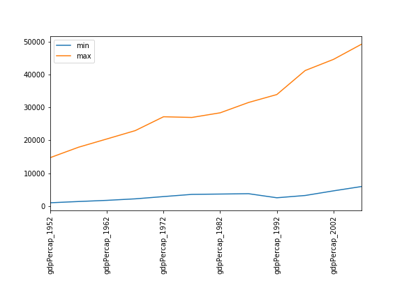
Minima and Maxima

Fill in the blanks below to plot the minimum GDP per capita over time for all the countries in Europe. Modify it again to plot the maximum GDP per capita over time for Europe.

data_europe = pd.read_csv('data/gapminder_gdp_europe.csv', index_col='country')
data_europe.____.plot(label='min')
data_europe.____
plt.legend(loc='best')
plt.xticks(rotation=90)

Solution

data_europe = pd.read_csv('data/gapminder_gdp_europe.csv', index_col='country')
data_europe.min().plot(label='min')
data_europe.max().plot(label='max')
plt.legend(loc='best')
plt.xticks(rotation=90)

Correlations

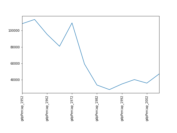
Modify the example in the notes to create a scatter plot showing the relationship between the minimum and maximum GDP per capita among the countries in Asia for each year in the data set. What relationship do you see (if any)?

Solution

data_asia = pd.read_csv('data/gapminder_gdp_asia.csv', index_col='country')
data_asia.describe().T.plot(kind='scatter', x='min', y='max')

No particular correlations can be seen between the minimum and maximum gdp values year on year. It seems the fortunes of asian countries do not rise and fall together.

You might note that the variability in the maximum is much higher than that of the minimum. Take a look at the maximum and the max indexes:

data_asia = pd.read_csv('data/gapminder_gdp_asia.csv', index_col='country')
data_asia.max().plot()
print(data_asia.idxmax())
print(data_asia.idxmin())

Solution

Seems the variability in this value is due to a sharp drop after 1972. Some geopolitics at play perhaps? Given the dominance of oil producing countries, maybe the Brent crude index would make an interesting comparison? Whilst Myanmar consistently has the lowest gdp, the highest gdb nation has varied more notably.

More Correlations

This short program creates a plot showing the correlation between GDP and life expectancy for 2007, normalizing marker size by population:

data_all = pd.read_csv('data/gapminder_all.csv', index_col='country')
data_all.plot(kind='scatter', x='gdpPercap_2007', y='lifeExp_2007',
              s=data_all['pop_2007']/1e6)

Using online help and other resources, explain what each argument to plot does.

Solution

A good place to look is the documentation for the plot function - help(data_all.plot).

kind - As seen already this determines the kind of plot to be drawn.

x and y - A column name or index that determines what data will be placed on the x and y axes of the plot

s - Details for this can be found in the documentation of plt.scatter. A single number or one value for each data point. Determines the size of the plotted points.

Saving your plot to a file

If you are satisfied with the plot you see you may want to save it to a file, perhaps to include it in a publication. There is a function in the matplotlib.pyplot module that accomplishes this: savefig. Calling this function, e.g. with

plt.savefig('my_figure.png')

will save the current figure to the file my_figure.png. The file format will automatically be deduced from the file name extension (other formats are pdf, ps, eps and svg).

Note that functions in plt refer to a global figure variable and after a figure has been displayed to the screen (e.g. with plt.show) matplotlib will make this variable refer to a new empty figure. Therefore, make sure you call plt.savefig before the plot is displayed to the screen, otherwise you may find a file with an empty plot.

When using dataframes, data is often generated and plotted to screen in one line, and plt.savefig seems not to be a possible approach. One possibility to save the figure to file is then to

• save a reference to the current figure in a local variable (with plt.gcf)
• call the savefig class method from that variable.

fig = plt.gcf() # get current figure
data.plot(kind='bar')
fig.savefig('my_figure.png')

Making your plots accessible

Whenever you are generating plots to go into a paper or a presentation, there are a few things you can do to make sure that everyone can understand your plots.

• Always make sure your text is large enough to read. Use the fontsize parameter in xlabel, ylabel, title, and legend, and tick_params with labelsize to increase the text size of the numbers on your axes.
• Similarly, you should make your graph elements easy to see. Use s to increase the size of your scatterplot markers and linewidth to increase the sizes of your plot lines.
• Using color (and nothing else) to distinguish between different plot elements will make your plots unreadable to anyone who is colorblind, or who happens to have a black-and-white office printer. For lines, the linestyle parameter lets you use different types of lines. For scatterplots, marker lets you change the shape of your points. If you’re unsure about your colors, you can use Coblis or Color Oracle to simulate what your plots would look like to those with colorblindness.

Key Points

• matplotlib is the most widely used scientific plotting library in Python.

• Plot data directly from a Pandas dataframe.

• Select and transform data, then plot it.

• Many styles of plot are available: see the Python Graph Gallery for more options.

• Can plot many sets of data together.

Storing Multiple Values in Lists

Overview

Teaching: 30 min
Exercises: 15 min

Questions

• How can I store many values together?

Objectives

• Explain what a list is.

• Create and index lists of simple values.

• Change the values of individual elements

• Append values to an existing list

• Reorder and slice list elements

• Create and manipulate nested lists

In the previous episode, we analyzed a single file with gapminder data. Our goal, however, is to process all the gapminder data we have, which means that we still have eleven more files to go!

The natural first step is to collect the names of all the files that we have to process. In Python, a list is a way to store multiple values together. In this episode, we will learn how to store multiple values in a list as well as how to work with lists.

Python lists

Unlike when we used pandas, lists are built into the language so we do not have to load a library to use them. We create a list by putting values inside square brackets and separating the values with commas:

odds = [1, 3, 5, 7]
print('odds are:', odds)

odds are: [1, 3, 5, 7]

We can access elements of a list using indices – numbered positions of elements in the list. These positions are numbered starting at 0, so the first element has an index of 0.

print('first element:', odds[0])
print('last element:', odds[3])
print('"-1" element:', odds[-1])

first element: 1
last element: 7
"-1" element: 7

Yes, we can use negative numbers as indices in Python. When we do so, the index -1 gives us the last element in the list, -2 the second to last, and so on. Because of this, odds[3] and odds[-1] point to the same element here.

There is one important difference between lists and strings: we can change the values in a list, but we cannot change individual characters in a string. For example:

names = ['Curie', 'Darwing', 'Turing']  # typo in Darwin's name
print('names is originally:', names)
names[1] = 'Darwin'  # correct the name
print('final value of names:', names)

names is originally: ['Curie', 'Darwing', 'Turing']
final value of names: ['Curie', 'Darwin', 'Turing']

works, but:

name = 'Darwin'
name[0] = 'd'

---------------------------------------------------------------------------
TypeError                                 Traceback (most recent call last)
<ipython-input-8-220df48aeb2e> in <module>()
      1 name = 'Darwin'
----> 2 name[0] = 'd'

TypeError: 'str' object does not support item assignment

does not.

Ch-Ch-Ch-Ch-Changes

Data which can be modified in place is called mutable, while data which cannot be modified is called immutable. Strings and numbers are immutable. This does not mean that variables with string or number values are constants, but when we want to change the value of a string or number variable, we can only replace the old value with a completely new value.

Lists and arrays, on the other hand, are mutable: we can modify them after they have been created. We can change individual elements, append new elements, or reorder the whole list. For some operations, like sorting, we can choose whether to use a function that modifies the data in-place or a function that returns a modified copy and leaves the original unchanged.

Be careful when modifying data in-place. If two variables refer to the same list, and you modify the list value, it will change for both variables!

salsa = ['peppers', 'onions', 'cilantro', 'tomatoes']
my_salsa = salsa        # <-- my_salsa and salsa point to the *same* list data in memory
salsa[0] = 'hot peppers'
print('Ingredients in my salsa:', my_salsa)

Ingredients in my salsa: ['hot peppers', 'onions', 'cilantro', 'tomatoes']

If you want variables with mutable values to be independent, you must make a copy of the value when you assign it.

salsa = ['peppers', 'onions', 'cilantro', 'tomatoes']
my_salsa = list(salsa)        # <-- makes a *copy* of the list
salsa[0] = 'hot peppers'
print('Ingredients in my salsa:', my_salsa)

Ingredients in my salsa: ['peppers', 'onions', 'cilantro', 'tomatoes']

Because of pitfalls like this, code which modifies data in place can be more difficult to understand. However, it is often far more efficient to modify a large data structure in place than to create a modified copy for every small change. You should consider both of these aspects when writing your code.

Nested Lists

Since a list can contain any Python variables, it can even contain other lists.

For example, we could represent the products in the shelves of a small grocery shop:

x = [['pepper', 'zucchini', 'onion'],
     ['cabbage', 'lettuce', 'garlic'],
     ['apple', 'pear', 'banana']]

Here is a visual example of how indexing a list of lists x works:

Using the previously declared list x, these would be the results of the index operations shown in the image:

print([x[0]])

[['pepper', 'zucchini', 'onion']]

print(x[0])

['pepper', 'zucchini', 'onion']

print(x[0][0])

'pepper'

Thanks to Hadley Wickham for the image above.

Heterogeneous Lists

Lists in Python can contain elements of different types. Example:

sample_ages = [10, 12.5, 'Unknown']

There are many ways to change the contents of lists besides assigning new values to individual elements:

odds.append(11)
print('odds after adding a value:', odds)

odds after adding a value: [1, 3, 5, 7, 11]

removed_element = odds.pop(0)
print('odds after removing the first element:', odds)
print('removed_element:', removed_element)

odds after removing the first element: [3, 5, 7, 11]
removed_element: 1

odds.reverse()
print('odds after reversing:', odds)

odds after reversing: [11, 7, 5, 3]

While modifying in place, it is useful to remember that Python treats lists in a slightly counter-intuitive way.

As we saw earlier, when we modified the salsa list item in-place, if we make a list, (attempt to) copy it and then modify this list, we can cause all sorts of trouble. This also applies to modifying the list using the above functions:

odds = [1, 3, 5, 7]
primes = odds
primes.append(2)
print('primes:', primes)
print('odds:', odds)

primes: [1, 3, 5, 7, 2]
odds: [1, 3, 5, 7, 2]

This is because Python stores a list in memory, and then can use multiple names to refer to the same list. If all we want to do is copy a (simple) list, we can again use the list function, so we do not modify a list we did not mean to:

odds = [1, 3, 5, 7]
primes = list(odds)
primes.append(2)
print('primes:', primes)
print('odds:', odds)

primes: [1, 3, 5, 7, 2]
odds: [1, 3, 5, 7]

Subsets of lists and strings can be accessed by specifying ranges of values in brackets, similar to how we accessed ranges of positions in a NumPy array. This is commonly referred to as “slicing” the list/string.

binomial_name = 'Drosophila melanogaster'
group = binomial_name[0:10]
print('group:', group)

species = binomial_name[11:23]
print('species:', species)

chromosomes = ['X', 'Y', '2', '3', '4']
autosomes = chromosomes[2:5]
print('autosomes:', autosomes)

last = chromosomes[-1]
print('last:', last)

group: Drosophila
species: melanogaster
autosomes: ['2', '3', '4']
last: 4

Slicing From the End

Use slicing to access only the last four characters of a string or entries of a list.

string_for_slicing = 'Observation date: 02-Feb-2013'
list_for_slicing = [['fluorine', 'F'],
                    ['chlorine', 'Cl'],
                    ['bromine', 'Br'],
                    ['iodine', 'I'],
                    ['astatine', 'At']]

'2013'
[['chlorine', 'Cl'], ['bromine', 'Br'], ['iodine', 'I'], ['astatine', 'At']]

Would your solution work regardless of whether you knew beforehand the length of the string or list (e.g. if you wanted to apply the solution to a set of lists of different lengths)? If not, try to change your approach to make it more robust.

Hint: Remember that indices can be negative as well as positive

Solution

Use negative indices to count elements from the end of a container (such as list or string):

string_for_slicing[-4:]
list_for_slicing[-4:]

Non-Continuous Slices

So far we’ve seen how to use slicing to take single blocks of successive entries from a sequence. But what if we want to take a subset of entries that aren’t next to each other in the sequence?

You can achieve this by providing a third argument to the range within the brackets, called the step size. The example below shows how you can take every third entry in a list:

primes = [2, 3, 5, 7, 11, 13, 17, 19, 23, 29, 31, 37]
subset = primes[0:12:3]
print('subset', subset)

subset [2, 7, 17, 29]

Notice that the slice taken begins with the first entry in the range, followed by entries taken at equally-spaced intervals (the steps) thereafter. If you wanted to begin the subset with the third entry, you would need to specify that as the starting point of the sliced range:

primes = [2, 3, 5, 7, 11, 13, 17, 19, 23, 29, 31, 37]
subset = primes[2:12:3]
print('subset', subset)

subset [5, 13, 23, 37]

Use the step size argument to create a new string that contains only every other character in the string “In an octopus’s garden in the shade”. Start with creating a variable to hold the string:

beatles = "In an octopus's garden in the shade"

What slice of beatles will produce the following output (i.e., the first character, third character, and every other character through the end of the string)?

I notpssgre ntesae

Solution

To obtain every other character you need to provide a slice with the step size of 2:

beatles[0:35:2]

You can also leave out the beginning and end of the slice to take the whole string and provide only the step argument to go every second element:

beatles[::2]

If you want to take a slice from the beginning of a sequence, you can omit the first index in the range:

date = 'Monday 4 January 2016'
day = date[0:6]
print('Using 0 to begin range:', day)
day = date[:6]
print('Omitting beginning index:', day)

Using 0 to begin range: Monday
Omitting beginning index: Monday

And similarly, you can omit the ending index in the range to take a slice to the very end of the sequence:

months = ['jan', 'feb', 'mar', 'apr', 'may', 'jun', 'jul', 'aug', 'sep', 'oct', 'nov', 'dec']
sond = months[8:12]
print('With known last position:', sond)
sond = months[8:len(months)]
print('Using len() to get last entry:', sond)
sond = months[8:]
print('Omitting ending index:', sond)

With known last position: ['sep', 'oct', 'nov', 'dec']
Using len() to get last entry: ['sep', 'oct', 'nov', 'dec']
Omitting ending index: ['sep', 'oct', 'nov', 'dec']

Overloading

+ usually means addition, but when used on strings or lists, it means “concatenate”. Given that, what do you think the multiplication operator * does on lists? In particular, what will be the output of the following code?

counts = [2, 4, 6, 8, 10]
repeats = counts * 2
print(repeats)

1. [2, 4, 6, 8, 10, 2, 4, 6, 8, 10]
2. [4, 8, 12, 16, 20]
3. [[2, 4, 6, 8, 10],[2, 4, 6, 8, 10]]
4. [2, 4, 6, 8, 10, 4, 8, 12, 16, 20]

The technical term for this is operator overloading: a single operator, like + or *, can do different things depending on what it’s applied to.

Solution

The multiplication operator * used on a list replicates elements of the list and concatenates them together:

[2, 4, 6, 8, 10, 2, 4, 6, 8, 10]

It’s equivalent to:

counts + counts

Key Points

• [value1, value2, value3, ...] creates a list.

• Lists can contain any Python object, including lists (i.e., list of lists).

• Lists are indexed and sliced with square brackets (e.g., list[0] and list[2:9]), in the same way as strings and arrays.

• Lists are mutable (i.e., their values can be changed in place).

• Strings are immutable (i.e., the characters in them cannot be changed).

Repeating Actions with Loops

Overview

Teaching: 30 min
Exercises: 10 min

Questions

• How can I do the same operations on many different values?

Objectives

• Explain what a for loop does.

• Correctly write for loops to repeat simple calculations.

• Trace changes to a loop variable as the loop runs.

• Trace changes to other variables as they are updated by a for loop.

An example task that we might want to repeat is accessing numbers in a list, which we will do by printing each number on a line of its own.

odds = [1, 3, 5, 7]

In Python, a list is basically an ordered collection of elements, and every element has a unique number associated with it — its index. This means that we can access elements in a list using their indices. For example, we can get the first number in the list odds, by using odds[0]. One way to print each number is to use four print statements:

print(odds[0])
print(odds[1])
print(odds[2])
print(odds[3])

1
3
5
7

This is a bad approach for three reasons:

1. Not scalable. Imagine you need to print a list that has hundreds of elements. It might be easier to type them in manually.

2. Difficult to maintain. If we want to decorate each printed element with an asterisk or any other character, we would have to change four lines of code. While this might not be a problem for small lists, it would definitely be a problem for longer ones.

3. Fragile. If we use it with a list that has more elements than what we initially envisioned, it will only display part of the list’s elements. A shorter list, on the other hand, will cause an error because it will be trying to display elements of the list that do not exist.

odds = [1, 3, 5]
print(odds[0])
print(odds[1])
print(odds[2])
print(odds[3])

1
3
5

---------------------------------------------------------------------------
IndexError                                Traceback (most recent call last)
<ipython-input-3-7974b6cdaf14> in <module>()
      3 print(odds[1])
      4 print(odds[2])
----> 5 print(odds[3])

IndexError: list index out of range

Here’s a better approach: a for loop

odds = [1, 3, 5, 7]
for num in odds:
    print(num)

1
3
5
7

This is shorter — certainly shorter than something that prints every number in a hundred-number list — and more robust as well:

odds = [1, 3, 5, 7, 9, 11]
for num in odds:
    print(num)

1
3
5
7
9
11

The improved version uses a for loop to repeat an operation — in this case, printing — once for each thing in a sequence. The general form of a loop is:

for variable in collection:
    # do things using variable, such as print

Using the odds example above, the loop might look like this:

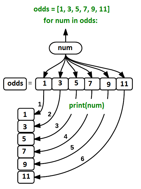
where each number (num) in the variable odds is looped through and printed one number after another. The other numbers in the diagram denote which loop cycle the number was printed in (1 being the first loop cycle, and 6 being the final loop cycle).

We can call the loop variable anything we like, but there must be a colon at the end of the line starting the loop, and we must indent anything we want to run inside the loop. Unlike many other languages, there is no command to signify the end of the loop body (e.g. end for); what is indented after the for statement belongs to the loop.

What’s in a name?

In the example above, the loop variable was given the name num as a mnemonic; it is short for ‘number’. We can choose any name we want for variables. We might just as easily have chosen the name banana for the loop variable, as long as we use the same name when we invoke the variable inside the loop:

odds = [1, 3, 5, 7, 9, 11]
for banana in odds:
    print(banana)

1
3
5
7
9
11

It is a good idea to choose variable names that are meaningful, otherwise it would be more difficult to understand what the loop is doing.

Here’s another loop that repeatedly updates a variable:

length = 0
names = ['Curie', 'Darwin', 'Turing']
for value in names:
    length = length + 1
print('There are', length, 'names in the list.')

There are 3 names in the list.

It’s worth tracing the execution of this little program step by step. Since there are three names in names, the statement on line 4 will be executed three times. The first time around, length is zero (the value assigned to it on line 1) and value is Curie. The statement adds 1 to the old value of length, producing 1, and updates length to refer to that new value. The next time around, value is Darwin and length is 1, so length is updated to be 2. After one more update, length is 3; since there is nothing left in names for Python to process, the loop finishes and the print function on line 5 tells us our final answer.

Note that a loop variable is a variable that is being used to record progress in a loop. It still exists after the loop is over, and we can re-use variables previously defined as loop variables as well:

name = 'Rosalind'
for name in ['Curie', 'Darwin', 'Turing']:
    print(name)
print('after the loop, name is', name)

Curie
Darwin
Turing
after the loop, name is Turing

Note also that finding the length of an object is such a common operation that Python actually has a built-in function to do it called len:

print(len([0, 1, 2, 3]))

4

len is much faster than any function we could write ourselves, and much easier to read than a two-line loop; it will also give us the length of many other things that we haven’t met yet, so we should always use it when we can.

From 1 to N

Python has a built-in function called range that generates a sequence of numbers. range can accept 1, 2, or 3 parameters.

• If one parameter is given, range generates a sequence of that length, starting at zero and incrementing by 1. For example, range(3) produces the numbers 0, 1, 2.
• If two parameters are given, range starts at the first and ends just before the second, incrementing by one. For example, range(2, 5) produces 2, 3, 4.
• If range is given 3 parameters, it starts at the first one, ends just before the second one, and increments by the third one. For example, range(3, 10, 2) produces 3, 5, 7, 9.

Using range, write a loop that uses range to print the first 3 natural numbers:

1
2
3

Solution

for number in range(1, 4):
    print(number)

Understanding the loops

Given the following loop:

word = 'oxygen'
for char in word:
    print(char)

How many times is the body of the loop executed?

• 3 times
• 4 times
• 5 times
• 6 times

Solution

The body of the loop is executed 6 times.

Computing Powers With Loops

Exponentiation is built into Python:

print(5 ** 3)

125

Write a loop that calculates the same result as 5 ** 3 using multiplication (and without exponentiation).

Solution

result = 1
for number in range(0, 3):
    result = result * 5
print(result)

Summing a list

Write a loop that calculates the sum of elements in a list by adding each element and printing the final value, so [124, 402, 36] prints 562

Solution

numbers = [124, 402, 36]
summed = 0
for num in numbers:
    summed = summed + num
print(summed)

Computing the Value of a Polynomial

The built-in function enumerate takes a sequence (e.g. a list) and generates a new sequence of the same length. Each element of the new sequence is a pair composed of the index (0, 1, 2,…) and the value from the original sequence:

for idx, val in enumerate(a_list):
    # Do something using idx and val

The code above loops through a_list, assigning the index to idx and the value to val.

Suppose you have encoded a polynomial as a list of coefficients in the following way: the first element is the constant term, the second element is the coefficient of the linear term, the third is the coefficient of the quadratic term, etc.

x = 5
coefs = [2, 4, 3]
y = coefs[0] * x**0 + coefs[1] * x**1 + coefs[2] * x**2
print(y)

97

Write a loop using enumerate(coefs) which computes the value y of any polynomial, given x and coefs.

Solution

y = 0
for idx, coef in enumerate(coefs):
    y = y + coef * x**idx

Key Points

• Use for variable in sequence to process the elements of a sequence one at a time.

• The body of a for loop must be indented.

• Use len(thing) to determine the length of something that contains other values.

Analyzing Data From Multiple Files

Overview

Teaching: 20 min
Exercises: 10 min

Questions

• How can I do the same operations on many different files?

Objectives

• Use a library function to get a list of filenames that match a wildcard pattern.

• Write a for loop to process multiple files.

Use a for loop to process files given a list of their names.

• A filename is a character string.
• And lists can contain character strings.

import pandas as pd
for filename in ['data/gapminder_gdp_africa.csv', 'data/gapminder_gdp_asia.csv']:
    data = pd.read_csv(filename, index_col='country')
    print(filename, data.min())

data/gapminder_gdp_africa.csv gdpPercap_1952    298.846212
gdpPercap_1957    335.997115
gdpPercap_1962    355.203227
gdpPercap_1967    412.977514
⋮ ⋮ ⋮
gdpPercap_1997    312.188423
gdpPercap_2002    241.165877
gdpPercap_2007    277.551859
dtype: float64
data/gapminder_gdp_asia.csv gdpPercap_1952    331
gdpPercap_1957    350
gdpPercap_1962    388
gdpPercap_1967    349
⋮ ⋮ ⋮
gdpPercap_1997    415
gdpPercap_2002    611
gdpPercap_2007    944
dtype: float64

Use glob.glob to find sets of files whose names match a pattern.

• In Unix, the term “globbing” means “matching a set of files with a pattern”.
• The most common patterns are:
  • * meaning “match zero or more characters”
  • ? meaning “match exactly one character”
• Python’s standard library contains the glob module to provide pattern matching functionality
• The glob module contains a function also called glob to match file patterns
• E.g., glob.glob('*.txt') matches all files in the current directory whose names end with .txt.
• Result is a (possibly empty) list of character strings.

import glob
print('all csv files in data directory:', glob.glob('data/*.csv'))

all csv files in data directory: ['data/gapminder_all.csv', 'data/gapminder_gdp_africa.csv', \
'data/gapminder_gdp_americas.csv', 'data/gapminder_gdp_asia.csv', 'data/gapminder_gdp_europe.csv', \
'data/gapminder_gdp_oceania.csv']

print('all PDB files:', glob.glob('*.pdb'))

all PDB files: []

Use glob and for to process batches of files.

• Helps a lot if the files are named and stored systematically and consistently so that simple patterns will find the right data.

for filename in glob.glob('data/gapminder_*.csv'):
    data = pd.read_csv(filename)
    print(filename, data['gdpPercap_1952'].min())

data/gapminder_all.csv 298.8462121
data/gapminder_gdp_africa.csv 298.8462121
data/gapminder_gdp_americas.csv 1397.717137
data/gapminder_gdp_asia.csv 331.0
data/gapminder_gdp_europe.csv 973.5331948
data/gapminder_gdp_oceania.csv 10039.59564

• This includes all data, as well as per-region data.
• Use a more specific pattern in the exercises to exclude the whole data set.
• But note that the minimum of the entire data set is also the minimum of one of the data sets, which is a nice check on correctness.

** TODO add example here of using wildcard to generate a plot from multiple files **

Determining Matches

Which of these files is not matched by the expression glob.glob('data/*as*.csv')?

1. data/gapminder_gdp_africa.csv
2. data/gapminder_gdp_americas.csv
3. data/gapminder_gdp_asia.csv

Solution

1 is not matched by the glob.

Minimum File Size

Modify this program so that it prints the number of records in the file that has the fewest records.

import glob
import pandas as pd
fewest = ____
for filename in glob.glob('data/*.csv'):
    dataframe = pd.____(filename)
    fewest = min(____, dataframe.shape[0])
print('smallest file has', fewest, 'records')

Note that the DataFrame.shape() method returns a tuple with the number of rows and columns of the data frame.

Solution

import glob
import pandas as pd
fewest = float('Inf')
for filename in glob.glob('data/*.csv'):
    dataframe = pd.read_csv(filename)
    fewest = min(fewest, dataframe.shape[0])
print('smallest file has', fewest, 'records')

Comparing Data

Write a program that reads in the regional data sets and plots the average GDP per capita for each region over time in a single chart.

Solution

This solution builds a useful legend by using the string split method to extract the region from the path ‘data/gapminder_gdp_a_specific_region.csv’.

import glob
import pandas as pd
import matplotlib.pyplot as plt
fig, ax = plt.subplots(1,1)
for filename in glob.glob('data/gapminder_gdp*.csv'):
    dataframe = pd.read_csv(filename)
    # extract {region} from the filename, expected to be in the format 'data/gapminder_gdp_{region}.csv'.
    # we will split the string using the split method and `_` as our separator,
    # retrieve the last string in the list that split returns (`{region}.csv`), 
    # and then remove the `.csv` extension from that string.
    region = filename.split('_')[-1][:-4] 
   # pandas raises errors when it encounters non-numeric columns in a dataframe computation
   # but we can tell pandas to ignore them with the `numeric_only` parameter
    dataframe.mean(numeric_only=True).plot(ax=ax, label=region)
plt.legend()
plt.show()

Dealing with File Paths

The pathlib module provides useful abstractions for file and path manipulation like returning the name of a file without the file extension. This is very useful when looping over files and directories. In the example below, we create a Path object and inspect its attributes.

from pathlib import Path

p = Path("data/gapminder_gdp_africa.csv")
print(p.parent), print(p.stem), print(p.suffix)

data
gapminder_gdp_africa
.csv

Hint: It is possible to check all available attributes and methods on the Path object with the dir() function!

Key Points

• Use glob.glob(pattern) to create a list of files whose names match a pattern.

• Use * in a pattern to match zero or more characters, and ? to match any single character.

Making Choices

Overview

Teaching: 30 min
Exercises: 10 min

Questions

• How can my programs do different things based on data values?

Objectives

• Write conditional statements including if, elif, and else branches.

• Correctly evaluate expressions containing and and or.

Conditionals

We can ask Python to take different actions, depending on a condition, with an if statement:

num = 37
if num > 100:
    print('greater')
else:
    print('not greater')
print('done')

not greater
done

The second line of this code uses the keyword if to tell Python that we want to make a choice. If the test that follows the if statement is true, the body of the if (i.e., the set of lines indented underneath it) is executed, and “greater” is printed. If the test is false, the body of the else is executed instead, and “not greater” is printed. Only one or the other is ever executed before continuing on with program execution to print “done”:

Conditional statements don’t have to include an else. If there isn’t one, Python simply does nothing if the test is false:

num = 53
print('before conditional...')
if num > 100:
    print(num, 'is greater than 100')
print('...after conditional')

before conditional...
...after conditional

We can also chain several tests together using elif, which is short for “else if”. The following Python code uses elif to print the sign of a number.

num = -3

if num > 0:
    print(num, 'is positive')
elif num == 0:
    print(num, 'is zero')
else:
    print(num, 'is negative')

-3 is negative

Note that to test for equality we use a double equals sign == rather than a single equals sign = which is used to assign values.

Comparing in Python

Along with the > and == operators we have already used for comparing values in our conditionals, there are a few more options to know about:

• >: greater than
• <: less than
• ==: equal to
• !=: does not equal
• >=: greater than or equal to
• <=: less than or equal to

We can also combine tests using and and or. and is only true if both parts are true:

if (1 > 0) and (-1 >= 0):
    print('both parts are true')
else:
    print('at least one part is false')

at least one part is false

while or is true if at least one part is true:

if (1 < 0) or (1 >= 0):
    print('at least one test is true')

at least one test is true

True and False

True and False are special words in Python called booleans, which represent truth values. A statement such as 1 < 0 returns the value False, while -1 < 0 returns the value True.

How Many Paths?

Consider this code:

if 4 > 5:
    print('A')
elif 4 == 5:
    print('B')
elif 4 < 5:
    print('C')

Which of the following would be printed if you were to run this code? Why did you pick this answer?

1. A
2. B
3. C
4. B and C

Solution

C gets printed because the first two conditions, 4 > 5 and 4 == 5, are not true, but 4 < 5 is true.

What Is Truth?

True and False booleans are not the only values in Python that are true and false. In fact, any value can be used in an if or elif. After reading and running the code below, explain what the rule is for which values are considered true and which are considered false.

if '':
    print('empty string is true')
if 'word':
    print('word is true')
if []:
    print('empty list is true')
if [1, 2, 3]:
    print('non-empty list is true')
if 0:
    print('zero is true')
if 1:
    print('one is true')

That’s Not Not What I Meant

Sometimes it is useful to check whether some condition is not true. The Boolean operator not can do this explicitly. After reading and running the code below, write some if statements that use not to test the rule that you formulated in the previous challenge.

if not '':
    print('empty string is not true')
if not 'word':
    print('word is not true')
if not not True:
    print('not not True is true')

Close Enough

Write some conditions that print True if the variable a is within 10% of the variable b and False otherwise. Compare your implementation with your partner’s: do you get the same answer for all possible pairs of numbers?

Hint

There is a built-in function abs that returns the absolute value of a number:

print(abs(-12))

12

Solution 1

a = 5
b = 5.1

if abs(a - b) <= 0.1 * abs(b):
    print('True')
else:
    print('False')

Solution 2

print(abs(a - b) <= 0.1 * abs(b))

This works because the Booleans True and False have string representations which can be printed.

In-Place Operators

Python (and most other languages in the C family) provides in-place operators that work like this:

x = 1  # original value
x += 1 # add one to x, assigning result back to x
x *= 3 # multiply x by 3
print(x)

6

Write some code that sums the positive and negative numbers in a list separately, using in-place operators. Do you think the result is more or less readable than writing the same without in-place operators?

Solution

positive_sum = 0
negative_sum = 0
test_list = [3, 4, 6, 1, -1, -5, 0, 7, -8]
for num in test_list:
    if num > 0:
        positive_sum += num
    elif num == 0:
        pass
    else:
        negative_sum += num
print(positive_sum, negative_sum)

Here pass means “don’t do anything”. In this particular case, it’s not actually needed, since if num == 0 neither sum needs to change, but it illustrates the use of elif and pass.

Counting Vowels

1. Write a loop that counts the number of vowels in a character string.
2. Test it on a few individual words and full sentences.
3. Once you are done, compare your solution to your neighbor’s. Did you make the same decisions about how to handle the letter ‘y’ (which some people think is a vowel, and some do not)?

Solution

vowels = 'aeiouAEIOU'
sentence = 'Mary had a little lamb.'
count = 0
for char in sentence:
    if char in vowels:
        count += 1

print('The number of vowels in this string is ' + str(count))

Key Points

• Use if condition to start a conditional statement, elif condition to provide additional tests, and else to provide a default.

• The bodies of the branches of conditional statements must be indented.

• Use == to test for equality.

• X and Y is only true if both X and Y are true.

• X or Y is true if either X or Y, or both, are true.

• Zero, the empty string, and the empty list are considered false; all other numbers, strings, and lists are considered true.

• True and False represent truth values.

Creating Functions

Overview

Teaching: 30 min
Exercises: 10 min

Questions

• How can I define new functions?

• What’s the difference between defining and calling a function?

• What happens when I call a function?

Objectives

• Define a function that takes parameters.

• Return a value from a function.

• Test and debug a function.

• Set default values for function parameters.

• Explain why we should divide programs into small, single-purpose functions.

Our code is getting pretty long and complicated; what if we had thousands of datasets, and didn’t want to generate a figure for every single one? Commenting out the figure-drawing code is a nuisance. Also, what if we want to use that code again, on a different dataset or at a different point in our program? Cutting and pasting it is going to make our code get very long and very repetitive, very quickly. We’d like a way to package our code so that it is easier to reuse, and Python provides for this by letting us define things called ‘functions’ — a shorthand way of re-executing longer pieces of code. Let’s start by defining a function fahr_to_celsius that converts temperatures from Fahrenheit to Celsius:

def fahr_to_celsius(temp):
    return ((temp - 32) * (5/9))

The function definition opens with the keyword def followed by the name of the function (fahr_to_celsius) and a parenthesized list of parameter names (temp). The body of the function — the statements that are executed when it runs — is indented below the definition line. The body concludes with a return keyword followed by the return value.

When we call the function, the values we pass to it are assigned to those variables so that we can use them inside the function. Inside the function, we use a return statement to send a result back to whoever asked for it.

Let’s try running our function.

fahr_to_celsius(32)

This command should call our function, using “32” as the input and return the function value.

In fact, calling our own function is no different from calling any other function:

print('freezing point of water:', fahr_to_celsius(32), 'C')
print('boiling point of water:', fahr_to_celsius(212), 'C')

freezing point of water: 0.0 C
boiling point of water: 100.0 C

We’ve successfully called the function that we defined, and we have access to the value that we returned.

Composing Functions

Now that we’ve seen how to turn Fahrenheit into Celsius, we can also write the function to turn Celsius into Kelvin:

def celsius_to_kelvin(temp_c):
    return temp_c + 273.15

print('freezing point of water in Kelvin:', celsius_to_kelvin(0.))

freezing point of water in Kelvin: 273.15

What about converting Fahrenheit to Kelvin? We could write out the formula, but we don’t need to. Instead, we can compose the two functions we have already created:

def fahr_to_kelvin(temp_f):
    temp_c = fahr_to_celsius(temp_f)
    temp_k = celsius_to_kelvin(temp_c)
    return temp_k

print('boiling point of water in Kelvin:', fahr_to_kelvin(212.0))

boiling point of water in Kelvin: 373.15

This is our first taste of how larger programs are built: we define basic operations, then combine them in ever-larger chunks to get the effect we want. Real-life functions will usually be larger than the ones shown here — typically half a dozen to a few dozen lines — but they shouldn’t ever be much longer than that, or the next person who reads it won’t be able to understand what’s going on.

Variable Scope

In composing our temperature conversion functions, we created variables inside of those functions, temp, temp_c, temp_f, and temp_k. We refer to these variables as local variables because they no longer exist once the function is done executing. If we try to access their values outside of the function, we will encounter an error:

print('Again, temperature in Kelvin was:', temp_k)

---------------------------------------------------------------------------
NameError                                 Traceback (most recent call last)
<ipython-input-1-eed2471d229b> in <module>
----> 1 print('Again, temperature in Kelvin was:', temp_k)

NameError: name 'temp_k' is not defined

If you want to reuse the temperature in Kelvin after you have calculated it with fahr_to_kelvin, you can store the result of the function call in a variable:

temp_kelvin = fahr_to_kelvin(212.0)
print('temperature in Kelvin was:', temp_kelvin)

temperature in Kelvin was: 373.15

The variable temp_kelvin, being defined outside any function, is said to be global.

Inside a function, one can read the value of such global variables:

def print_temperatures():
  print('temperature in Fahrenheit was:', temp_fahr)
  print('temperature in Kelvin was:', temp_kelvin)

temp_fahr = 212.0
temp_kelvin = fahr_to_kelvin(temp_fahr)

print_temperatures()

temperature in Fahrenheit was: 212.0
temperature in Kelvin was: 373.15

Now that we know how to wrap bits of code up in functions, we can make our inflammation analysis easier to read and easier to reuse. First, let’s make a visualize function that generates our plots:

import matplotlib.pyplot as plt
def visualize(filename):
    data = pd.read_csv(filename, index_col='country')
    fig, ax = plt.subplots(1, 2, figsize=(12.0, 5.0))
    
    data.columns = data.columns.str.strip('gdpPercap_')

    ax[0].set_ylabel(data.index[0])
    ax[0].plot(data.loc[data.index[0]])
    ax[1].set_ylabel(data.index[1])
    ax[1].plot(data.loc[data.index[1]])
    
    fig.tight_layout()
    plt.show()

Wait! Didn’t we forget to specify what both of these functions should return? Well, we didn’t. In Python, functions are not required to include a return statement and can be used for the sole purpose of grouping together pieces of code that conceptually do one thing. In such cases, function names usually describe what they do, e.g. visualize.

Notice that rather than jumbling this code together in one giant for loop, we can now read and reuse both ideas separately. We can reproduce the previous analysis with a much simpler for loop:

filenames = sorted(glob.glob('data/gapminder_gdp_a[fs]*.csv'))

for filename in filenames:
    print(filename)
    visualize(filename)

By giving our functions human-readable names, we can more easily read and understand what is happening in the for loop. Even better, if at some later date we want to use either of those pieces of code again, we can do so in a single line.

Readable functions

Consider these two functions:

def s(p):
    a = 0
    for v in p:
        a += v
    m = a / len(p)
    d = 0
    for v in p:
        d += (v - m) * (v - m)
    return numpy.sqrt(d / (len(p) - 1))

def std_dev(sample):
    sample_sum = 0
    for value in sample:
        sample_sum += value

    sample_mean = sample_sum / len(sample)

    sum_squared_devs = 0
    for value in sample:
        sum_squared_devs += (value - sample_mean) * (value - sample_mean)

    return numpy.sqrt(sum_squared_devs / (len(sample) - 1))

The functions s and std_dev are computationally equivalent (they both calculate the sample standard deviation), but to a human reader, they look very different. You probably found std_dev much easier to read and understand than s.

As this example illustrates, both documentation and a programmer’s coding style combine to determine how easy it is for others to read and understand the programmer’s code. Choosing meaningful variable names and using blank spaces to break the code into logical “chunks” are helpful techniques for producing readable code. This is useful not only for sharing code with others, but also for the original programmer. If you need to revisit code that you wrote months ago and haven’t thought about since then, you will appreciate the value of readable code!

Combining Strings

“Adding” two strings produces their concatenation: 'a' + 'b' is 'ab'. Write a function called fence that takes two parameters called original and wrapper and returns a new string that has the wrapper character at the beginning and end of the original. A call to your function should look like this:

print(fence('name', '*'))

*name*

Solution

def fence(original, wrapper):
    return wrapper + original + wrapper

Return versus print

Note that return and print are not interchangeable. print is a Python function that prints data to the screen. It enables us, users, see the data. return statement, on the other hand, makes data visible to the program. Let’s have a look at the following function:

def add(a, b):
    print(a + b)

Question: What will we see if we execute the following commands?

A = add(7, 3)
print(A)

Solution

Python will first execute the function add with a = 7 and b = 3, and, therefore, print 10. However, because function add does not have a line that starts with return (no return “statement”), it will, by default, return nothing which, in Python world, is called None. Therefore, A will be assigned to None and the last line (print(A)) will print None. As a result, we will see:

10
None

Selecting Characters From Strings

If the variable s refers to a string, then s[0] is the string’s first character and s[-1] is its last. Write a function called outer that returns a string made up of just the first and last characters of its input. A call to your function should look like this:

print(outer('helium'))

hm

Solution

def outer(input_string):
    return input_string[0] + input_string[-1]

Rescaling an Array

Write a function rescale that takes an array as input and returns a corresponding array of values scaled to lie in the range 0.0 to 1.0. (Hint: If L and H are the lowest and highest values in the original array, then the replacement for a value v should be (v-L) / (H-L).)

Solution

def rescale(input_array):
    L = numpy.min(input_array)
    H = numpy.max(input_array)
    output_array = (input_array - L) / (H - L)
    return output_array

Testing and Documenting Your Function

Run the commands help(numpy.arange) and help(numpy.linspace) to see how to use these functions to generate regularly-spaced values, then use those values to test your rescale function. Once you’ve successfully tested your function, add a docstring that explains what it does.

Solution

"""Takes an array as input, and returns a corresponding array scaled so
that 0 corresponds to the minimum and 1 to the maximum value of the input array.

Examples:
>>> rescale(numpy.arange(10.0))
array([ 0.        ,  0.11111111,  0.22222222,  0.33333333,  0.44444444,
       0.55555556,  0.66666667,  0.77777778,  0.88888889,  1.        ])
>>> rescale(numpy.linspace(0, 100, 5))
array([ 0.  ,  0.25,  0.5 ,  0.75,  1.  ])
"""

Defining Defaults

Rewrite the rescale function so that it scales data to lie between 0.0 and 1.0 by default, but will allow the caller to specify lower and upper bounds if they want. Compare your implementation to your neighbor’s: do the two functions always behave the same way?

Solution

def rescale(input_array, low_val=0.0, high_val=1.0):
    """rescales input array values to lie between low_val and high_val"""
    L = numpy.min(input_array)
    H = numpy.max(input_array)
    intermed_array = (input_array - L) / (H - L)
    output_array = intermed_array * (high_val - low_val) + low_val
    return output_array

Variables Inside and Outside Functions

What does the following piece of code display when run — and why?

f = 0
k = 0

def f2k(f):
    k = ((f - 32) * (5.0 / 9.0)) + 273.15
    return k

print(f2k(8))
print(f2k(41))
print(f2k(32))

print(k)

Solution

259.81666666666666
278.15
273.15
0

k is 0 because the k inside the function f2k doesn’t know about the k defined outside the function. When the f2k function is called, it creates a local variable k. The function does not return any values and does not alter k outside of its local copy. Therefore the original value of k remains unchanged. Beware that a local k is created because f2k internal statements affect a new value to it. If k was only read, it would simply retreive the global k value.

Mixing Default and Non-Default Parameters

Given the following code:

def numbers(one, two=2, three, four=4):
    n = str(one) + str(two) + str(three) + str(four)
    return n

print(numbers(1, three=3))

what do you expect will be printed? What is actually printed? What rule do you think Python is following?

1. 1234
2. one2three4
3. 1239
4. SyntaxError

Given that, what does the following piece of code display when run?

def func(a, b=3, c=6):
    print('a: ', a, 'b: ', b, 'c:', c)

func(-1, 2)

1. a: b: 3 c: 6
2. a: -1 b: 3 c: 6
3. a: -1 b: 2 c: 6
4. a: b: -1 c: 2

Solution

Attempting to define the numbers function results in 4. SyntaxError. The defined parameters two and four are given default values. Because one and three are not given default values, they are required to be included as arguments when the function is called and must be placed before any parameters that have default values in the function definition.

The given call to func displays a: -1 b: 2 c: 6. -1 is assigned to the first parameter a, 2 is assigned to the next parameter b, and c is not passed a value, so it uses its default value 6.

Readable Code

Revise a function you wrote for one of the previous exercises to try to make the code more readable. Then, collaborate with one of your neighbors to critique each other’s functions and discuss how your function implementations could be further improved to make them more readable.

Key Points

• Define a function using def function_name(parameter).

• The body of a function must be indented.

• Call a function using function_name(value).

• Numbers are stored as integers or floating-point numbers.

• Variables defined within a function can only be seen and used within the body of the function.

• Variables created outside of any function are called global variables.

• Within a function, we can access global variables.

• Variables created within a function override global variables if their names match.

• Use help(thing) to view help for something.

• Put docstrings in functions to provide help for that function.

• Specify default values for parameters when defining a function using name=value in the parameter list.

• Parameters can be passed by matching based on name, by position, or by omitting them (in which case the default value is used).

• Put code whose parameters change frequently in a function, then call it with different parameter values to customize its behavior.

Errors and Exceptions

Overview

Teaching: 30 min
Exercises: 10 min

Questions

• How does Python report errors?

• How can I handle errors in Python programs?

Objectives

• To be able to read a traceback, and determine where the error took place and what type it is.

• To be able to describe the types of situations in which syntax errors, indentation errors, name errors, index errors, and missing file errors occur.

Every programmer encounters errors, both those who are just beginning, and those who have been programming for years. Encountering errors and exceptions can be very frustrating at times, and can make coding feel like a hopeless endeavour. However, understanding what the different types of errors are and when you are likely to encounter them can help a lot. Once you know why you get certain types of errors, they become much easier to fix.

Errors in Python have a very specific form, called a traceback. Let’s examine one:

# This code has an intentional error. You can type it directly or
# use it for reference to understand the error message below.
def favorite_ice_cream():
    ice_creams = [
        'chocolate',
        'vanilla',
        'strawberry'
    ]
    print(ice_creams[3])

favorite_ice_cream()

---------------------------------------------------------------------------
IndexError                                Traceback (most recent call last)
<ipython-input-1-70bd89baa4df> in <module>()
      9     print(ice_creams[3])
      10
----> 11 favorite_ice_cream()

<ipython-input-1-70bd89baa4df> in favorite_ice_cream()
      7         'strawberry'
      8     ]
----> 9     print(ice_creams[3])
      10
      11 favorite_ice_cream()

IndexError: list index out of range

This particular traceback has two levels. You can determine the number of levels by looking for the number of arrows on the left hand side. In this case:

1. The first shows code from the cell above, with an arrow pointing to Line 11 (which is favorite_ice_cream()).

2. The second shows some code in the function favorite_ice_cream, with an arrow pointing to Line 9 (which is print(ice_creams[3])).

The last level is the actual place where the error occurred. The other level(s) show what function the program executed to get to the next level down. So, in this case, the program first performed a function call to the function favorite_ice_cream. Inside this function, the program encountered an error on Line 6, when it tried to run the code print(ice_creams[3]).

Long Tracebacks

Sometimes, you might see a traceback that is very long – sometimes they might even be 20 levels deep! This can make it seem like something horrible happened, but the length of the error message does not reflect severity, rather, it indicates that your program called many functions before it encountered the error. Most of the time, the actual place where the error occurred is at the bottom-most level, so you can skip down the traceback to the bottom.

So what error did the program actually encounter? In the last line of the traceback, Python helpfully tells us the category or type of error (in this case, it is an IndexError) and a more detailed error message (in this case, it says “list index out of range”).

If you encounter an error and don’t know what it means, it is still important to read the traceback closely. That way, if you fix the error, but encounter a new one, you can tell that the error changed. Additionally, sometimes knowing where the error occurred is enough to fix it, even if you don’t entirely understand the message.

If you do encounter an error you don’t recognize, try looking at the official documentation on errors. However, note that you may not always be able to find the error there, as it is possible to create custom errors. In that case, hopefully the custom error message is informative enough to help you figure out what went wrong.

Syntax Errors

When you forget a colon at the end of a line, accidentally add one space too many when indenting under an if statement, or forget a parenthesis, you will encounter a syntax error. This means that Python couldn’t figure out how to read your program. This is similar to forgetting punctuation in English: for example, this text is difficult to read there is no punctuation there is also no capitalization why is this hard because you have to figure out where each sentence ends you also have to figure out where each sentence begins to some extent it might be ambiguous if there should be a sentence break or not

People can typically figure out what is meant by text with no punctuation, but people are much smarter than computers. If Python doesn’t know how to read the program, it will give up and inform you with an error. For example:

def some_function()
    msg = 'hello, world!'
    print(msg)
     return msg

  File "<ipython-input-3-6bb841ea1423>", line 1
    def some_function()
                       ^
SyntaxError: invalid syntax

Here, Python tells us that there is a SyntaxError on line 1, and even puts a little arrow in the place where there is an issue. In this case the problem is that the function definition is missing a colon at the end.

Actually, the function above has two issues with syntax. If we fix the problem with the colon, we see that there is also an IndentationError, which means that the lines in the function definition do not all have the same indentation:

def some_function():
    msg = 'hello, world!'
    print(msg)
     return msg

  File "<ipython-input-4-ae290e7659cb>", line 4
    return msg
    ^
IndentationError: unexpected indent

Both SyntaxError and IndentationError indicate a problem with the syntax of your program, but an IndentationError is more specific: it always means that there is a problem with how your code is indented.

Tabs and Spaces

Some indentation errors are harder to spot than others. In particular, mixing spaces and tabs can be difficult to spot because they are both whitespace. In the example below, the first two lines in the body of the function some_function are indented with tabs, while the third line — with spaces. If you’re working in a Jupyter notebook, be sure to copy and paste this example rather than trying to type it in manually because Jupyter automatically replaces tabs with spaces.

def some_function():
	msg = 'hello, world!'
	print(msg)
        return msg

Visually it is impossible to spot the error. Fortunately, Python does not allow you to mix tabs and spaces.

  File "<ipython-input-5-653b36fbcd41>", line 4
    return msg
              ^
TabError: inconsistent use of tabs and spaces in indentation

Variable Name Errors

Another very common type of error is called a NameError, and occurs when you try to use a variable that does not exist. For example:

print(a)

---------------------------------------------------------------------------
NameError                                 Traceback (most recent call last)
<ipython-input-7-9d7b17ad5387> in <module>()
----> 1 print(a)

NameError: name 'a' is not defined

Variable name errors come with some of the most informative error messages, which are usually of the form “name ‘the_variable_name’ is not defined”.

Why does this error message occur? That’s a harder question to answer, because it depends on what your code is supposed to do. However, there are a few very common reasons why you might have an undefined variable. The first is that you meant to use a string, but forgot to put quotes around it:

print(hello)

---------------------------------------------------------------------------
NameError                                 Traceback (most recent call last)
<ipython-input-8-9553ee03b645> in <module>()
----> 1 print(hello)

NameError: name 'hello' is not defined

The second reason is that you might be trying to use a variable that does not yet exist. In the following example, count should have been defined (e.g., with count = 0) before the for loop:

for number in range(10):
    count = count + number
print('The count is:', count)

---------------------------------------------------------------------------
NameError                                 Traceback (most recent call last)
<ipython-input-9-dd6a12d7ca5c> in <module>()
      1 for number in range(10):
----> 2     count = count + number
      3 print('The count is:', count)

NameError: name 'count' is not defined

Finally, the third possibility is that you made a typo when you were writing your code. Let’s say we fixed the error above by adding the line Count = 0 before the for loop. Frustratingly, this actually does not fix the error. Remember that variables are case-sensitive, so the variable count is different from Count. We still get the same error, because we still have not defined count:

Count = 0
for number in range(10):
    count = count + number
print('The count is:', count)

---------------------------------------------------------------------------
NameError                                 Traceback (most recent call last)
<ipython-input-10-d77d40059aea> in <module>()
      1 Count = 0
      2 for number in range(10):
----> 3     count = count + number
      4 print('The count is:', count)

NameError: name 'count' is not defined

Index Errors

Next up are errors having to do with containers (like lists and strings) and the items within them. If you try to access an item in a list or a string that does not exist, then you will get an error. This makes sense: if you asked someone what day they would like to get coffee, and they answered “caturday”, you might be a bit annoyed. Python gets similarly annoyed if you try to ask it for an item that doesn’t exist:

letters = ['a', 'b', 'c']
print('Letter #1 is', letters[0])
print('Letter #2 is', letters[1])
print('Letter #3 is', letters[2])
print('Letter #4 is', letters[3])

Letter #1 is a
Letter #2 is b
Letter #3 is c

---------------------------------------------------------------------------
IndexError                                Traceback (most recent call last)
<ipython-input-11-d817f55b7d6c> in <module>()
      3 print('Letter #2 is', letters[1])
      4 print('Letter #3 is', letters[2])
----> 5 print('Letter #4 is', letters[3])

IndexError: list index out of range

Here, Python is telling us that there is an IndexError in our code, meaning we tried to access a list index that did not exist.

File Errors

The last type of error we’ll cover today are those associated with reading and writing files: FileNotFoundError. If you try to read a file that does not exist, you will receive a FileNotFoundError telling you so. If you attempt to write to a file that was opened read-only, Python 3 returns an UnsupportedOperationError. More generally, problems with input and output manifest as IOErrors or OSErrors, depending on the version of Python you use.

file_handle = open('myfile.txt', 'r')

---------------------------------------------------------------------------
FileNotFoundError                         Traceback (most recent call last)
<ipython-input-14-f6e1ac4aee96> in <module>()
----> 1 file_handle = open('myfile.txt', 'r')

FileNotFoundError: [Errno 2] No such file or directory: 'myfile.txt'

One reason for receiving this error is that you specified an incorrect path to the file. For example, if I am currently in a folder called myproject, and I have a file in myproject/writing/myfile.txt, but I try to open myfile.txt, this will fail. The correct path would be writing/myfile.txt. It is also possible that the file name or its path contains a typo.

A related issue can occur if you use the “read” flag instead of the “write” flag. Python will not give you an error if you try to open a file for writing when the file does not exist. However, if you meant to open a file for reading, but accidentally opened it for writing, and then try to read from it, you will get an UnsupportedOperation error telling you that the file was not opened for reading:

file_handle = open('myfile.txt', 'w')
file_handle.read()

---------------------------------------------------------------------------
UnsupportedOperation                      Traceback (most recent call last)
<ipython-input-15-b846479bc61f> in <module>()
      1 file_handle = open('myfile.txt', 'w')
----> 2 file_handle.read()

UnsupportedOperation: not readable

These are the most common errors with files, though many others exist. If you get an error that you’ve never seen before, searching the Internet for that error type often reveals common reasons why you might get that error.

Reading Error Messages

Read the Python code and the resulting traceback below, and answer the following questions:

1. How many levels does the traceback have?
2. What is the function name where the error occurred?
3. On which line number in this function did the error occur?
4. What is the type of error?
5. What is the error message?

# This code has an intentional error. Do not type it directly;
# use it for reference to understand the error message below.
def print_message(day):
    messages = {
        'monday': 'Hello, world!',
        'tuesday': 'Today is Tuesday!',
        'wednesday': 'It is the middle of the week.',
        'thursday': 'Today is Donnerstag in German!',
        'friday': 'Last day of the week!',
        'saturday': 'Hooray for the weekend!',
        'sunday': 'Aw, the weekend is almost over.'
    }
    print(messages[day])

def print_friday_message():
    print_message('Friday')

print_friday_message()

---------------------------------------------------------------------------
KeyError                                  Traceback (most recent call last)
<ipython-input-1-4be1945adbe2> in <module>()
     14     print_message('Friday')
     15
---> 16 print_friday_message()

<ipython-input-1-4be1945adbe2> in print_friday_message()
     12
     13 def print_friday_message():
---> 14     print_message('Friday')
     15
     16 print_friday_message()

<ipython-input-1-4be1945adbe2> in print_message(day)
      9         'sunday': 'Aw, the weekend is almost over.'
     10     }
---> 11     print(messages[day])
     12
     13 def print_friday_message():

KeyError: 'Friday'

Solution

1. 3 levels
2. print_message
3. 11
4. KeyError
5. There isn’t really a message; you’re supposed to infer that Friday is not a key in messages.

Identifying Syntax Errors

1. Read the code below, and (without running it) try to identify what the errors are.
2. Run the code, and read the error message. Is it a SyntaxError or an IndentationError?
3. Fix the error.
4. Repeat steps 2 and 3, until you have fixed all the errors.

def another_function
  print('Syntax errors are annoying.')
   print('But at least Python tells us about them!')
  print('So they are usually not too hard to fix.')

Solution

SyntaxError for missing (): at end of first line, IndentationError for mismatch between second and third lines. A fixed version is:

def another_function():
    print('Syntax errors are annoying.')
    print('But at least Python tells us about them!')
    print('So they are usually not too hard to fix.')

Identifying Variable Name Errors

1. Read the code below, and (without running it) try to identify what the errors are.
2. Run the code, and read the error message. What type of NameError do you think this is? In other words, is it a string with no quotes, a misspelled variable, or a variable that should have been defined but was not?
3. Fix the error.
4. Repeat steps 2 and 3, until you have fixed all the errors.

for number in range(10):
    # use a if the number is a multiple of 3, otherwise use b
    if (Number % 3) == 0:
        message = message + a
    else:
        message = message + 'b'
print(message)

Solution

3 NameErrors for number being misspelled, for message not defined, and for a not being in quotes.

Fixed version:

message = ''
for number in range(10):
    # use a if the number is a multiple of 3, otherwise use b
    if (number % 3) == 0:
        message = message + 'a'
    else:
        message = message + 'b'
print(message)

Identifying Index Errors

1. Read the code below, and (without running it) try to identify what the errors are.
2. Run the code, and read the error message. What type of error is it?
3. Fix the error.

seasons = ['Spring', 'Summer', 'Fall', 'Winter']
print('My favorite season is ', seasons[4])

Solution

IndexError; the last entry is seasons[3], so seasons[4] doesn’t make sense. A fixed version is:

seasons = ['Spring', 'Summer', 'Fall', 'Winter']
print('My favorite season is ', seasons[-1])

Key Points

• Tracebacks can look intimidating, but they give us a lot of useful information about what went wrong in our program, including where the error occurred and what type of error it was.

• An error having to do with the ‘grammar’ or syntax of the program is called a SyntaxError. If the issue has to do with how the code is indented, then it will be called an IndentationError.

• A NameError will occur when trying to use a variable that does not exist. Possible causes are that a variable definition is missing, a variable reference differs from its definition in spelling or capitalization, or the code contains a string that is missing quotes around it.

• Containers like lists and strings will generate errors if you try to access items in them that do not exist. This type of error is called an IndexError.

• Trying to read a file that does not exist will give you an FileNotFoundError. Trying to read a file that is open for writing, or writing to a file that is open for reading, will give you an IOError.

Defensive Programming

Overview

Teaching: 30 min
Exercises: 10 min

Questions

• How can I make my programs more reliable?

Objectives

• Explain what an assertion is.

• Add assertions that check the program’s state is correct.

• Correctly add precondition and postcondition assertions to functions.

• Explain what test-driven development is, and use it when creating new functions.

• Explain why variables should be initialized using actual data values rather than arbitrary constants.

Our previous lessons have introduced the basic tools of programming: variables and lists, file I/O, loops, conditionals, and functions. What they haven’t done is show us how to tell whether a program is getting the right answer, and how to tell if it’s still getting the right answer as we make changes to it.

To achieve that, we need to:

• Write programs that check their own operation.
• Write and run tests for widely-used functions.
• Make sure we know what “correct” actually means.

The good news is, doing these things will speed up our programming, not slow it down. As in real carpentry — the kind done with lumber — the time saved by measuring carefully before cutting a piece of wood is much greater than the time that measuring takes.

Assertions

The first step toward getting the right answers from our programs is to assume that mistakes will happen and to guard against them. This is called defensive programming, and the most common way to do it is to add assertions to our code so that it checks itself as it runs. An assertion is simply a statement that something must be true at a certain point in a program. When Python sees one, it evaluates the assertion’s condition. If it’s true, Python does nothing, but if it’s false, Python halts the program immediately and prints the error message if one is provided. For example, this piece of code halts as soon as the loop encounters a value that isn’t positive:

numbers = [1.5, 2.3, 0.7, -0.001, 4.4]
total = 0.0
for num in numbers:
    assert num > 0.0, 'Data should only contain positive values'
    total += num
print('total is:', total)

---------------------------------------------------------------------------
AssertionError                            Traceback (most recent call last)
<ipython-input-19-33d87ea29ae4> in <module>()
      2 total = 0.0
      3 for num in numbers:
----> 4     assert num > 0.0, 'Data should only contain positive values'
      5     total += num
      6 print('total is:', total)

AssertionError: Data should only contain positive values

Programs like the Firefox browser are full of assertions: 10-20% of the code they contain are there to check that the other 80–90% are working correctly. Broadly speaking, assertions fall into three categories:

• A precondition is something that must be true at the start of a function in order for it to work correctly.

• A postcondition is something that the function guarantees is true when it finishes.

• An invariant is something that is always true at a particular point inside a piece of code.

For example, suppose we are representing rectangles using a tuple of four coordinates (x0, y0, x1, y1), representing the lower left and upper right corners of the rectangle. In order to do some calculations, we need to normalize the rectangle so that the lower left corner is at the origin and the longest side is 1.0 units long. This function does that, but checks that its input is correctly formatted and that its result makes sense:

def normalize_rectangle(rect):
    """Normalizes a rectangle so that it is at the origin and 1.0 units long on its longest axis.
    Input should be of the format (x0, y0, x1, y1).
    (x0, y0) and (x1, y1) define the lower left and upper right corners
    of the rectangle, respectively."""
    assert len(rect) == 4, 'Rectangles must contain 4 coordinates'
    x0, y0, x1, y1 = rect
    assert x0 < x1, 'Invalid X coordinates'
    assert y0 < y1, 'Invalid Y coordinates'

    dx = x1 - x0
    dy = y1 - y0
    if dx > dy:
        scaled = float(dx) / dy
        upper_x, upper_y = 1.0, scaled
    else:
        scaled = float(dx) / dy
        upper_x, upper_y = scaled, 1.0

    assert 0 < upper_x <= 1.0, 'Calculated upper X coordinate invalid'
    assert 0 < upper_y <= 1.0, 'Calculated upper Y coordinate invalid'

    return (0, 0, upper_x, upper_y)

The preconditions on lines 6, 8, and 9 catch invalid inputs:

print(normalize_rectangle( (0.0, 1.0, 2.0) )) # missing the fourth coordinate

---------------------------------------------------------------------------
AssertionError                            Traceback (most recent call last)
<ipython-input-2-1b9cd8e18a1f> in <module>
----> 1 print(normalize_rectangle( (0.0, 1.0, 2.0) )) # missing the fourth coordinate

<ipython-input-1-c94cf5b065b9> in normalize_rectangle(rect)
      4     (x0, y0) and (x1, y1) define the lower left and upper right corners
      5     of the rectangle, respectively."""
----> 6     assert len(rect) == 4, 'Rectangles must contain 4 coordinates'
      7     x0, y0, x1, y1 = rect
      8     assert x0 < x1, 'Invalid X coordinates'

AssertionError: Rectangles must contain 4 coordinates

print(normalize_rectangle( (4.0, 2.0, 1.0, 5.0) )) # X axis inverted

---------------------------------------------------------------------------
AssertionError                            Traceback (most recent call last)
<ipython-input-3-325036405532> in <module>
----> 1 print(normalize_rectangle( (4.0, 2.0, 1.0, 5.0) )) # X axis inverted

<ipython-input-1-c94cf5b065b9> in normalize_rectangle(rect)
      6     assert len(rect) == 4, 'Rectangles must contain 4 coordinates'
      7     x0, y0, x1, y1 = rect
----> 8     assert x0 < x1, 'Invalid X coordinates'
      9     assert y0 < y1, 'Invalid Y coordinates'
     10

AssertionError: Invalid X coordinates

The post-conditions on lines 20 and 21 help us catch bugs by telling us when our calculations might have been incorrect. For example, if we normalize a rectangle that is taller than it is wide everything seems OK:

print(normalize_rectangle( (0.0, 0.0, 1.0, 5.0) ))

(0, 0, 0.2, 1.0)

but if we normalize one that’s wider than it is tall, the assertion is triggered:

print(normalize_rectangle( (0.0, 0.0, 5.0, 1.0) ))

---------------------------------------------------------------------------
AssertionError                            Traceback (most recent call last)
<ipython-input-5-8d4a48f1d068> in <module>
----> 1 print(normalize_rectangle( (0.0, 0.0, 5.0, 1.0) ))

<ipython-input-1-c94cf5b065b9> in normalize_rectangle(rect)
     19
     20     assert 0 < upper_x <= 1.0, 'Calculated upper X coordinate invalid'
---> 21     assert 0 < upper_y <= 1.0, 'Calculated upper Y coordinate invalid'
     22
     23     return (0, 0, upper_x, upper_y)

AssertionError: Calculated upper Y coordinate invalid

Re-reading our function, we realize that line 14 should divide dy by dx rather than dx by dy. In a Jupyter notebook, you can display line numbers by typing Ctrl+M followed by L. If we had left out the assertion at the end of the function, we would have created and returned something that had the right shape as a valid answer, but wasn’t. Detecting and debugging that would almost certainly have taken more time in the long run than writing the assertion.

But assertions aren’t just about catching errors: they also help people understand programs. Each assertion gives the person reading the program a chance to check (consciously or otherwise) that their understanding matches what the code is doing.

Most good programmers follow two rules when adding assertions to their code. The first is, fail early, fail often. The greater the distance between when and where an error occurs and when it’s noticed, the harder the error will be to debug, so good code catches mistakes as early as possible.

The second rule is, turn bugs into assertions or tests. Whenever you fix a bug, write an assertion that catches the mistake should you make it again. If you made a mistake in a piece of code, the odds are good that you have made other mistakes nearby, or will make the same mistake (or a related one) the next time you change it. Writing assertions to check that you haven’t regressed (i.e., haven’t re-introduced an old problem) can save a lot of time in the long run, and helps to warn people who are reading the code (including your future self) that this bit is tricky.

Test-Driven Development

An assertion checks that something is true at a particular point in the program. The next step is to check the overall behavior of a piece of code, i.e., to make sure that it produces the right output when it’s given a particular input. For example, suppose we need to find where two or more time series overlap. The range of each time series is represented as a pair of numbers, which are the time the interval started and ended. The output is the largest range that they all include:

Most novice programmers would solve this problem like this:

1. Write a function range_overlap.
2. Call it interactively on two or three different inputs.
3. If it produces the wrong answer, fix the function and re-run that test.

This clearly works — after all, thousands of scientists are doing it right now — but there’s a better way:

1. Write a short function for each test.
2. Write a range_overlap function that should pass those tests.
3. If range_overlap produces any wrong answers, fix it and re-run the test functions.

Writing the tests before writing the function they exercise is called test-driven development (TDD). Its advocates believe it produces better code faster because:

1. If people write tests after writing the thing to be tested, they are subject to confirmation bias, i.e., they subconsciously write tests to show that their code is correct, rather than to find errors.
2. Writing tests helps programmers figure out what the function is actually supposed to do.

Here are three test functions for range_overlap:

assert range_overlap([ (0.0, 1.0) ]) == (0.0, 1.0)
assert range_overlap([ (2.0, 3.0), (2.0, 4.0) ]) == (2.0, 3.0)
assert range_overlap([ (0.0, 1.0), (0.0, 2.0), (-1.0, 1.0) ]) == (0.0, 1.0)

---------------------------------------------------------------------------
AssertionError                            Traceback (most recent call last)
<ipython-input-25-d8be150fbef6> in <module>()
----> 1 assert range_overlap([ (0.0, 1.0) ]) == (0.0, 1.0)
      2 assert range_overlap([ (2.0, 3.0), (2.0, 4.0) ]) == (2.0, 3.0)
      3 assert range_overlap([ (0.0, 1.0), (0.0, 2.0), (-1.0, 1.0) ]) == (0.0, 1.0)

AssertionError:

The error is actually reassuring: we haven’t written range_overlap yet, so if the tests passed, it would be a sign that someone else had and that we were accidentally using their function.

And as a bonus of writing these tests, we’ve implicitly defined what our input and output look like: we expect a list of pairs as input, and produce a single pair as output.

Something important is missing, though. We don’t have any tests for the case where the ranges don’t overlap at all:

assert range_overlap([ (0.0, 1.0), (5.0, 6.0) ]) == ???

What should range_overlap do in this case: fail with an error message, produce a special value like (0.0, 0.0) to signal that there’s no overlap, or something else? Any actual implementation of the function will do one of these things; writing the tests first helps us figure out which is best before we’re emotionally invested in whatever we happened to write before we realized there was an issue.

And what about this case?

assert range_overlap([ (0.0, 1.0), (1.0, 2.0) ]) == ???

Do two segments that touch at their endpoints overlap or not? Mathematicians usually say “yes”, but engineers usually say “no”. The best answer is “whatever is most useful in the rest of our program”, but again, any actual implementation of range_overlap is going to do something, and whatever it is ought to be consistent with what it does when there’s no overlap at all.

Since we’re planning to use the range this function returns as the X axis in a time series chart, we decide that:

1. every overlap has to have non-zero width, and
2. we will return the special value None when there’s no overlap.

None is built into Python, and means “nothing here”. (Other languages often call the equivalent value null or nil). With that decision made, we can finish writing our last two tests:

assert range_overlap([ (0.0, 1.0), (5.0, 6.0) ]) == None
assert range_overlap([ (0.0, 1.0), (1.0, 2.0) ]) == None

---------------------------------------------------------------------------
AssertionError                            Traceback (most recent call last)
<ipython-input-26-d877ef460ba2> in <module>()
----> 1 assert range_overlap([ (0.0, 1.0), (5.0, 6.0) ]) == None
      2 assert range_overlap([ (0.0, 1.0), (1.0, 2.0) ]) == None

AssertionError:

Again, we get an error because we haven’t written our function, but we’re now ready to do so:

def range_overlap(ranges):
    """Return common overlap among a set of [left, right] ranges."""
    max_left = 0.0
    min_right = 1.0
    for (left, right) in ranges:
        max_left = max(max_left, left)
        min_right = min(min_right, right)
    return (max_left, min_right)

Take a moment to think about why we calculate the left endpoint of the overlap as the maximum of the input left endpoints, and the overlap right endpoint as the minimum of the input right endpoints. We’d now like to re-run our tests, but they’re scattered across three different cells. To make running them easier, let’s put them all in a function:

def test_range_overlap():
    assert range_overlap([ (0.0, 1.0), (5.0, 6.0) ]) == None
    assert range_overlap([ (0.0, 1.0), (1.0, 2.0) ]) == None
    assert range_overlap([ (0.0, 1.0) ]) == (0.0, 1.0)
    assert range_overlap([ (2.0, 3.0), (2.0, 4.0) ]) == (2.0, 3.0)
    assert range_overlap([ (0.0, 1.0), (0.0, 2.0), (-1.0, 1.0) ]) == (0.0, 1.0)
    assert range_overlap([]) == None

We can now test range_overlap with a single function call:

test_range_overlap()

---------------------------------------------------------------------------
AssertionError                            Traceback (most recent call last)
<ipython-input-29-cf9215c96457> in <module>()
----> 1 test_range_overlap()

<ipython-input-28-5d4cd6fd41d9> in test_range_overlap()
      1 def test_range_overlap():
----> 2     assert range_overlap([ (0.0, 1.0), (5.0, 6.0) ]) == None
      3     assert range_overlap([ (0.0, 1.0), (1.0, 2.0) ]) == None
      4     assert range_overlap([ (0.0, 1.0) ]) == (0.0, 1.0)
      5     assert range_overlap([ (2.0, 3.0), (2.0, 4.0) ]) == (2.0, 3.0)

AssertionError:

The first test that was supposed to produce None fails, so we know something is wrong with our function. We don’t know whether the other tests passed or failed because Python halted the program as soon as it spotted the first error. Still, some information is better than none, and if we trace the behavior of the function with that input, we realize that we’re initializing max_left and min_right to 0.0 and 1.0 respectively, regardless of the input values. This violates another important rule of programming: always initialize from data.

Pre- and Post-Conditions

Suppose you are writing a function called average that calculates the average of the numbers in a list. What pre-conditions and post-conditions would you write for it? Compare your answer to your neighbor’s: can you think of a function that will pass your tests but not his/hers or vice versa?

Solution

# a possible pre-condition:
assert len(input_list) > 0, 'List length must be non-zero'
# a possible post-condition:
assert numpy.min(input_list) <= average <= numpy.max(input_list),
'Average should be between min and max of input values (inclusive)'

Testing Assertions

Given a sequence of a number of cars, the function get_total_cars returns the total number of cars.

get_total_cars([1, 2, 3, 4])

10

get_total_cars(['a', 'b', 'c'])

ValueError: invalid literal for int() with base 10: 'a'

Explain in words what the assertions in this function check, and for each one, give an example of input that will make that assertion fail.

def get_total(values):
    assert len(values) > 0
    for element in values:
        assert int(element)
    values = [int(element) for element in values]
    total = sum(values)
    assert total > 0
    return total

Solution

• The first assertion checks that the input sequence values is not empty. An empty sequence such as [] will make it fail.
• The second assertion checks that each value in the list can be turned into an integer. Input such as [1, 2,'c', 3] will make it fail.
• The third assertion checks that the total of the list is greater than 0. Input such as [-10, 2, 3] will make it fail.

Key Points

• Program defensively, i.e., assume that errors are going to arise, and write code to detect them when they do.

• Put assertions in programs to check their state as they run, and to help readers understand how those programs are supposed to work.

• Use preconditions to check that the inputs to a function are safe to use.

• Use postconditions to check that the output from a function is safe to use.

• Write tests before writing code in order to help determine exactly what that code is supposed to do.

Debugging

Overview

Teaching: 30 min
Exercises: 20 min

Questions

• How can I debug my program?

Objectives

• Debug code containing an error systematically.

• Identify ways of making code less error-prone and more easily tested.

Once testing has uncovered problems, the next step is to fix them. Many novices do this by making more-or-less random changes to their code until it seems to produce the right answer, but that’s very inefficient (and the result is usually only correct for the one case they’re testing). The more experienced a programmer is, the more systematically they debug, and most follow some variation on the rules explained below.

Know What It’s Supposed to Do

The first step in debugging something is to know what it’s supposed to do. “My program doesn’t work” isn’t good enough: in order to diagnose and fix problems, we need to be able to tell correct output from incorrect. If we can write a test case for the failing case — i.e., if we can assert that with these inputs, the function should produce that result — then we’re ready to start debugging. If we can’t, then we need to figure out how we’re going to know when we’ve fixed things.

But writing test cases for scientific software is frequently harder than writing test cases for commercial applications, because if we knew what the output of the scientific code was supposed to be, we wouldn’t be running the software: we’d be writing up our results and moving on to the next program. In practice, scientists tend to do the following:

1. Test with simplified data. Before doing statistics on a real data set, we should try calculating statistics for a single record, for two identical records, for two records whose values are one step apart, or for some other case where we can calculate the right answer by hand.

2. Test a simplified case. If our program is supposed to simulate magnetic eddies in rapidly-rotating blobs of supercooled helium, our first test should be a blob of helium that isn’t rotating, and isn’t being subjected to any external electromagnetic fields. Similarly, if we’re looking at the effects of climate change on speciation, our first test should hold temperature, precipitation, and other factors constant.

3. Compare to an oracle. A test oracle is something whose results are trusted, such as experimental data, an older program, or a human expert. We use test oracles to determine if our new program produces the correct results. If we have a test oracle, we should store its output for particular cases so that we can compare it with our new results as often as we like without re-running that program.

4. Check conservation laws. Mass, energy, and other quantities are conserved in physical systems, so they should be in programs as well. Similarly, if we are analyzing patient data, the number of records should either stay the same or decrease as we move from one analysis to the next (since we might throw away outliers or records with missing values). If “new” patients start appearing out of nowhere as we move through our pipeline, it’s probably a sign that something is wrong.

5. Visualize. Data analysts frequently use simple visualizations to check both the science they’re doing and the correctness of their code (just as we did in the opening lesson of this tutorial). This should only be used for debugging as a last resort, though, since it’s very hard to compare two visualizations automatically.