Autoregressive Integrated Moving Average Forecasts
Last updated on 2023-08-18 | Edit this page
Estimated time: 50 minutes
Overview
Questions
- How can we forecast non-stationary time-series?
Objectives
- Explain the d parameter of the SARIMAX model’s order(p, d, q) argument.
Introduction
The smart meter data with which we have been modeling forecasts throughout this lesson are non-stationary. That is, there are trends in the data. An assumption of the moving average and autoregressive models that we’ve looked at is that the data are stationary.
So far, we have been manually differencing the data and making forecasts with the differenced data, then transforming the forecasts back to the scale of the source dataset. In this section, we look at the autoregressive integrated moving average or ARIMA(p,d, q) model. In this model, as before, the p is the order of the AR(p) process and the q is the order of the MA(q) process. Now we will further specify the d parameter, which is the integration order.
About the code
The code used in this lesson is based on and, in some cases, a direct application of code used in the Manning Publications title, Time series forecasting in Python, by Marco Peixeiro.
Peixeiro, Marco. Time Series Forecasting in Python. [First edition]. Manning Publications Co., 2022.
The original code from the book is made available under an Apache 2.0 license. Use and application of the code in these materials is within the license terms, although this lesson itself is licensed under a Creative Commons CC-BY 4.0 license. Any further use or adaptation of these materials should cite the source code developed by Peixeiro:
Peixeiro, Marco. Timeseries Forecasting in Python [Software code]. 2022. Accessed from https://github.com/marcopeix/TimeSeriesForecastingInPython.
Create the data subset
In order to more fully demonstrate the integration order of the process, we are going to generate a different subset that needs to be differenced twice before it is stationary. That is, whereas all of our time-series so far have only required first order differencing to become stationary, this subset will require second order differencing.
First, import the required libraries.
PYTHON
import pandas as pd
import numpy as np
import matplotlib.pyplot as plt
from statsmodels.tsa.stattools import adfuller
from statsmodels.graphics.tsaplots import plot_acf
from statsmodels.graphics.tsaplots import plot_pacf
from statsmodels.tsa.statespace.sarimax import SARIMAX
from sklearn.metrics import mean_squared_error
from sklearn.metrics import mean_absolute_error
We will reuse our function for reading, subsetting, and resampling the data.
PYTHON
def subset_resample(fpath, sample_freq, start_date, end_date=None):
    df = pd.read_csv(fpath)
    df.set_index(pd.to_datetime(df["INTERVAL_TIME"]), inplace=True)
    df.sort_index(inplace=True)
    if end_date:
        date_subset = df.loc[start_date: end_date].copy()
    else:
        date_subset = df.loc[start_date].copy()
    resampled_data = date_subset.resample(sample_freq)
    return resampled_data
This time we call our function with different arguments for the file path and the date range of the subset.
PYTHON
fp = "../../data/ladpu_smart_meter_data_02.csv"
data_subset_resampled = subset_resample(fp, "D", "2019-04", end_date="2019-06")
print("Data type of returned object:", type(data_subset_resampled))
OUTPUT
Data type of returned object: <class 'pandas.core.resample.DatetimeIndexResampler'>The object returned by the subset_resample function is a
datetime group, so as before we create a dataframe from an aggregation
of the grouped statistics.
PYTHON
daily_usage = data_subset_resampled['INTERVAL_READ'].agg([np.sum])
print(daily_usage.info())
print(daily_usage.head())
OUTPUT
<class 'pandas.core.frame.DataFrame'>
DatetimeIndex: 91 entries, 2019-04-01 to 2019-06-30
Freq: D
Data columns (total 1 columns):
# Column Non-Null Count Dtype
--- ------ -------------- -----
0 sum 91 non-null float64
dtypes: float64(1)
memory usage: 1.4 KB
None
sum
INTERVAL_TIME
2019-04-01 10.4928
2019-04-02 13.8258
2019-04-03 9.1350
2019-04-04 15.8994
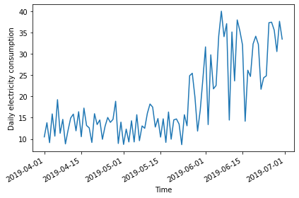
2019-04-05 10.6644Plot the data - the date range is smaller than previous examples, and there is a notable trend in increased power consumption toward the end of the date range.
Determine the integration order of the process
Not surprisingly, the AD Fuller statistic indicates that the time-series is not stationary.
PYTHON
ADF_result = adfuller(daily_usage['sum'])
print(f'ADF Statistic: {ADF_result[0]}')
print(f'p-value: {ADF_result[1]}')
OUTPUT
ADF Statistic: 0.043745771110572505
p-value: 0.9620037401385906
However, after differencing the data the AD Fuller statistic is lower but still indicates that the data are not stationary.
PYTHON
daily_usage_diff = np.diff(daily_usage['sum'], n = 1)

ADF_result = adfuller(daily_usage_diff)
print(f'ADF Statistic: {ADF_result[0]}')
print(f'p-value: {ADF_result[1]}')
OUTPUT
ADF Statistic: -2.552170893387957
p-value: 0.10329088087274496
If we difference the differenced data, the AD Fuller statistic and p-value now indicate that our time-series is stationary.
PYTHON
daily_usage_diff2 = np.diff(daily_usage_diff, n=1)

ad_fuller_result = adfuller(daily_usage_diff2)

print(f'ADF Statistic: {ad_fuller_result[0]}')
print(f'p-value: {ad_fuller_result[1]}')
OUTPUT
ADF Statistic: -11.308460105521412
p-value: 1.2561555209524703e-20
As noted, up until now we have been forecasting and fitting models with training data subset from the differenced time-series. Because we are now integration order to our model, we will be fitting models and making forecasts using the non-stationary source data.
Since we needed to use second order differencing to make our time-series stationary, the value d of the ARIMA(p, d, q) integration order is 2.
First, create training and test data sets.
PYTHON
train = daily_usage[:int(len(daily_usage) * .9)].copy() # ~90% of data
test = daily_usage[int(len(daily_usage) * .9):].copy() # ~10% of data
print("Training data length:", len(train))
print("Test data length:", len(test))
OUTPUT
Training data length: 81
Test data length: 10
Plot the time-series, with the forecast range shaded.
PYTHON
fig, (ax1) = plt.subplots(nrows=1, ncols=1, sharex=True, figsize=(10, 8))

ax1.plot(daily_usage['sum'].values)
ax1.set_xlabel('Time')
ax1.set_ylabel('Energy use')
ax1.axvspan(81, 91, color='#808080', alpha=0.2)

fig.autofmt_xdate()
plt.tight_layout()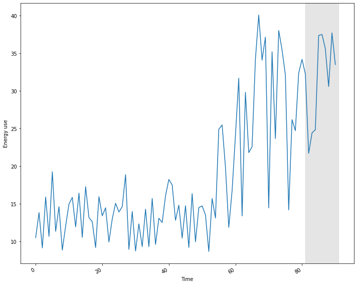
Determine the ARMA(p, q) orders of the process
In addition to the integration order, we also need to know the orders of the AR(p) and MA(q) processes. We can determine these using the Akaike information criterion, as before. The process is the same. First, we create a list of possible p and q values.
PYTHON
from itertools import product

p_vals = range(0, 4, 1)
q_vals = range(0, 4, 1)

order_list = list(product(p_vals, q_vals))

for o in order_list:
    print(o)
OUTPUT
(0, 0)
(0, 1)
(0, 2)
(0, 3)
(1, 0)
(1, 1)
(1, 2)
(1, 3)
(2, 0)
(2, 1)
(2, 2)
(2, 3)
(3, 0)
(3, 1)
(3, 2)
(3, 3)
Next, we reuse our function to fit models using each combination of ARMA(p, q) orders. Note that we have made a change to the function to include the integration order as an argument that is passed to the order argument of the SARIMAX model.
PYTHON
def fit_eval_AIC(data, order_list, i_order):
    aic_results = []
    for o in order_list:
        model = SARIMAX(data, order=(o[0], i_order, o[1]),
                        simple_differencing=False)
        res = model.fit(disp=False)
        aic = res.aic
        aic_results.append([o, aic])

    result_df = pd.DataFrame(aic_results, columns=(['(p, q)', 'AIC']))
    result_df.sort_values(by='AIC', ascending=True, inplace=True)
    result_df.reset_index(drop=True, inplace=True)

    return result_df
Passing our training data to a function call of our AIC evaluation function, the result indicates that the model with the best comparative performance has an ARMA(2, 3) process. Including the integration order gives us an optimized ARIMA(2, 2, 3) process.
OUTPUT
    (p, q)         AIC
0   (2, 3)  497.916050
1   (1, 3)  499.220250
2   (3, 3)  499.620967
3   (3, 2)  503.250113
4   (2, 2)  509.066593
5   (0, 2)  510.498182
6   (3, 1)  511.524737
7   (0, 3)  512.309653
8   (1, 2)  514.444378
9   (1, 1)  515.938985
10  (2, 1)  517.934902
11  (3, 0)  544.559757
12  (0, 1)  547.563212
13  (2, 0)  551.625374
14  (1, 0)  555.131203
15  (0, 0)  632.868700
Before forecasting, we still need to perform diagnostics to make sure
the model doesn’t violate any of its underlying assumptions. We can do
this using plot_diagnostics().
PYTHON
model = SARIMAX(train, order=(2,2,3), simple_differencing=False)
model_fit = model.fit(disp=False)
model_fit.plot_diagnostics(figsize=(10,8));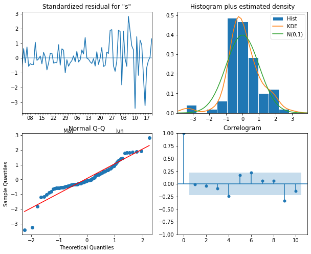
Forecast using an ARIMA(2, 2, 3) process
One advantage to using the non-stationary time-series to diagnose the optimized ARIMA(2, 2, 3) model is that predictions are an attribute of the corresponding SARIMAX model. That is, we don’t have to define a separate function to make forecasts.
First, in order to evaluate the forecasts from our ARIMA(2, 2, 3) model, we need to define a baseline. In this case since we are forecasting power consumption across the last ten days of the time-series, we will use a naive seasonal forecast, which is a pairwise forecast the uses the last ten values of the training set as the forecast for the ten values of the test set.
OUTPUT
                   sum  naive_seasonal
INTERVAL_TIME
2019-06-21     32.2602         35.1876
2019-06-22     21.7008         23.6634
2019-06-23     24.4098         38.0220
2019-06-24     24.8472         35.4414
2019-06-25     37.3656         32.1318
2019-06-26     37.4856         14.1774
2019-06-27     35.6100         26.1804
2019-06-28     30.5742         24.7188
2019-06-29     37.6950         32.3622
2019-06-30     33.4986         34.1838
Now we can use the get_prediction() method of the
SARIMAX model to retrieve the predicted power consumption over the ten
days of the test set.
PYTHON
pred_ARIMA = model_fit.get_prediction(81, 91).predicted_mean

# add these to a new column in test set
test['pred_ARIMA'] = pred_ARIMA
print(test)
OUTPUT
                   sum  naive_seasonal  pred_ARIMA
INTERVAL_TIME
2019-06-21     32.2602         35.1876   36.311936
2019-06-22     21.7008         23.6634   30.731745
2019-06-23     24.4098         38.0220   35.999676
2019-06-24     24.8472         35.4414   31.301976
2019-06-25     37.3656         32.1318   36.802939
2019-06-26     37.4856         14.1774   32.181567
2019-06-27     35.6100         26.1804   37.692010
2019-06-28     30.5742         24.7188   33.084946
2019-06-29     37.6950         32.3622   38.587688
2019-06-30     33.4986         34.1838   33.990146
Finally, we can evaluate the performance of the baseline and the model using the mean absolute error.
PYTHON
mae_naive_seasonal = mean_absolute_error(test['sum'], test['naive_seasonal'])
mae_ARIMA = mean_absolute_error(test['sum'], test['pred_ARIMA'])

print("Mean absolute error, baseline:", mae_naive_seasonal)
print("Mean absolute error, ARMA(2, 2, 3):", mae_ARIMA)
OUTPUT
Mean absolute error, baseline: 7.89414
Mean absolute error, ARMA(2, 2, 3): 4.297101587602739
We can visually compare the results using a plot.
PYTHON
fig, ax = plt.subplots()

ax.plot(daily_usage['sum'])
ax.plot(test['sum'], 'b-', label='actual')
ax.plot(test['naive_seasonal'], 'r:', label='naive seasonal')
ax.plot(test['pred_ARIMA'], 'k--', label='ARIMA(2,2,3)')

ax.set_xlabel('Date')
ax.set_ylabel('Electricity consumption')

ax.legend(loc=2)

fig.autofmt_xdate()
plt.tight_layout()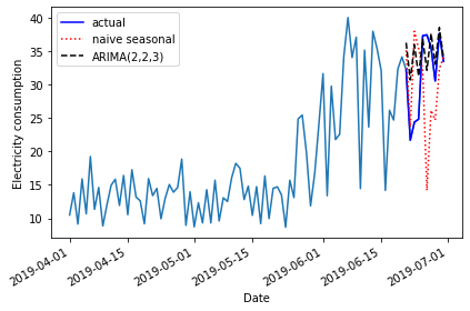
Key Points
- The d parameter of the order argument of the SARIMAX model can be used to forecast non-stationary time-series.