Autoregressive Moving Average Forecasts
Last updated on 2023-08-18 | Edit this page
Estimated time: 50 minutes
Overview
Questions
- How can we forecast time-series with both moving average and autoregressive processes?
Objectives
- Apply a generalized workflow to fit different models.
Introduction
Further refining process to combine parameters of order of processes.
About the code
The code used in this lesson is based on and, in some cases, a direct application of code used in the Manning Publications title, Time series forecasting in Python, by Marco Peixeiro.
Peixeiro, Marco. Time Series Forecasting in Python. [First edition]. Manning Publications Co., 2022.
The original code from the book is made available under an Apache 2.0 license. Use and application of the code in these materials is within the license terms, although this lesson itself is licensed under a Creative Commons CC-BY 4.0 license. Any further use or adaptation of these materials should cite the source code developed by Peixeiro:
Peixeiro, Marco. Timeseries Forecasting in Python [Software code]. 2022. Accessed from https://github.com/marcopeix/TimeSeriesForecastingInPython.
Read and subset data
Import libraries.
PYTHON
import pandas as pd
import numpy as np
import matplotlib.pyplot as plt
from statsmodels.tsa.stattools import adfuller
from statsmodels.graphics.tsaplots import plot_acf
from statsmodels.graphics.tsaplots import plot_pacf
from statsmodels.tsa.statespace.sarimax import SARIMAX
from sklearn.metrics import mean_squared_error
from sklearn.metrics import mean_absolute_error
Reuse our function to read, subset, and resample data.
PYTHON
def subset_resample(fpath, sample_freq, start_date, end_date=None):
    df = pd.read_csv(fpath)
    df.set_index(pd.to_datetime(df["INTERVAL_TIME"]), inplace=True)
    df.sort_index(inplace=True)
    if end_date:
        date_subset = df.loc[start_date: end_date].copy()
    else:
        date_subset = df.loc[start_date].copy()
    resampled_data = date_subset.resample(sample_freq)
    return resampled_data
Call the function.
PYTHON
fp = "../../data/ladpu_smart_meter_data_01.csv"
data_subset_resampled = subset_resample(fp, "D", "2019-01", end_date="2019-07")
print("Data type of returned object:", type(data_subset_resampled))
OUTPUT
Data type of returned object: <class 'pandas.core.resample.DatetimeIndexResampler'>Create a dataframe and inspect.
PYTHON
daily_usage = data_subset_resampled['INTERVAL_READ'].agg([np.sum])
print(daily_usage.info())
print(daily_usage.head())
OUTPUT
<class 'pandas.core.frame.DataFrame'>
DatetimeIndex: 212 entries, 2019-01-01 to 2019-07-31
Freq: D
Data columns (total 1 columns):
 #   Column  Non-Null Count  Dtype
---  ------  --------------  -----
 0   sum     212 non-null    float64
dtypes: float64(1)
memory usage: 3.3 KB
None
                   sum
INTERVAL_TIME
2019-01-01      7.5324
2019-01-02     10.2534
2019-01-03      6.8544
2019-01-04      5.3250
2019-01-05      7.5480
Plot.
PYTHON
fig, ax = plt.subplots()

ax.plot(daily_usage['sum'])
ax.set_xlabel('Time')
ax.set_ylabel('Daily electricity consumption')

fig.autofmt_xdate()
plt.tight_layout()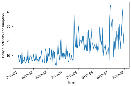
AD Fuller test.
PYTHON
adfuller_test = adfuller(daily_usage)
print(f'ADFuller result: {adfuller_test[0]}')
print(f'p-value: {adfuller_test[1]}')
OUTPUT
ADFuller result: -2.533089941397639
p-value: 0.10762933815081588
Difference data.
PYTHON
daily_usage_diff = np.diff(daily_usage['sum'], n = 1)
adfuller_test = adfuller(daily_usage_diff)
print(f'ADFuller result: {adfuller_test[0]}')
print(f'p-value: {adfuller_test[1]}')
OUTPUT
ADFuller result: -7.966077912452976
p-value: 2.8626643210939594e-12
Plot ACF
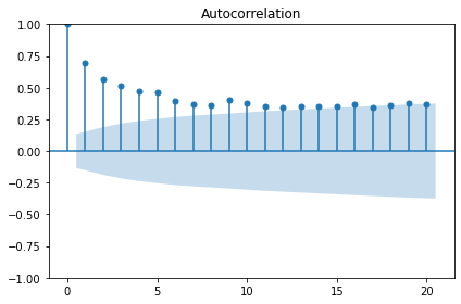
Determine the orders of the ARMA(p, q) processes
Plot indicates an autoregressive process.
The order of an autoregressive moving average, or ARMA, process, may not be intelligible from a PACF plot. For the remainder of this lesson, rather than determine order by visually inspecting plots we will statistically determine order of AR and MA processes using a generalized procedure.
We will fit multiple models with different values for the order of
the AR and MA processes and evaluate each one by the resulting Akaike
information criterion (AIC) value. The AIC is an attribute of a SARIMAX
model, so we will continue to refine our function for interacting with
the SARIMAX model of the statsmodel library.
First we create a list of possible values of the orders of the AR and MA processes. In the code below and in general use, the order of the AR process is given as p, while the order of the MA process is given as q.
PYTHON
from itertools import product

p_vals = range(0, 4, 1)
q_vals = range(0, 4, 1)

order_list = list(product(p_vals, q_vals))

for o in order_list:
    print(o)
OUTPUT
(0, 0)
(0, 1)
(0, 2)
(0, 3)
(1, 0)
(1, 1)
(1, 2)
(1, 3)
(2, 0)
(2, 1)
(2, 2)
(2, 3)
(3, 0)
(3, 1)
(3, 2)
(3, 3)
The output above demonstrates the combinations of AR(p) and MA(q) values we will be using to fit, in this case, 16 different ARMA(p, q) models. We will compare the AIC of the results and select the best performing model.
Since we’re not forecasting yet, we will write a new function to fit and evaluate our 16 models.
PYTHON
def fit_eval_AIC(data, order_list):
    aic_results = []
    for o in order_list:
        model = SARIMAX(data, order=(o[0], 0, o[1]),
                        simple_differencing=False)
        res = model.fit(disp=False)
        aic = res.aic
        aic_results.append([o, aic])

    result_df = pd.DataFrame(aic_results, columns=(['(p, q)', 'AIC']))
    result_df.sort_values(by='AIC', ascending=True, inplace=True)
    result_df.reset_index(drop=True, inplace=True)

    return result_df
The function will return a dataframe of ARMA(p, q) combinations and their corresponding AIC values. Results have been sorted by ascending AIC values since a lower AIC value is better. Generally, the top performing model will be listed first.
OUTPUT
(p, q) AIC
0 (1, 1) 1338.285936
1 (1, 2) 1340.280751
2 (2, 1) 1340.281961
3 (2, 2) 1341.021637
4 (0, 2) 1341.239402
5 (0, 3) 1341.295724
6 (3, 1) 1341.845466
7 (2, 3) 1342.689150
8 (3, 2) 1342.699834
9 (3, 3) 1342.905525
10 (1, 3) 1344.861937
11 (0, 1) 1356.044366
12 (3, 0) 1358.323315
13 (2, 0) 1363.368153
14 (1, 0) 1375.855521
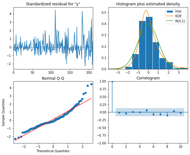
15 (0, 0) 1391.965311The result indicates that the best performing model among the 16 is
the ARMA(1, 1) model. But in a worst case this could simply mean that
the ARMA(1, 1) model is the least bad out of the models we fitted. We
also want to assess its overall quality. Before using the model to
forecast, it’s also perform diagnostics to make sure the model doesn’t
violate any of its underlying assumptions. We can use
plot_diagnostics() to evaluate the distribution of
residuals of the ARMA(1, 1) model.
PYTHON
model = SARIMAX(daily_usage_diff, order=(1,0,1), simple_differencing=False)
model_fit = model.fit(disp=False)
model_fit.plot_diagnostics(figsize=(10, 8));
The plots indicate that there is some room for improvement. We will see this improvement in a later section of this lesson when we finally account for the seasonal trends evident in the data. But for now we will proceed and show that the ARMA(p, q) process nonetheless represent a significant improvement over forecasting with either the AR(p) or MA(q) processes by themselves.
Forecast using an ARMA(p, q) model
In the previous section we already updated our forecasting function to initialize a SARIMAX model using variables for the AR(p) and MA(q) orders in the order argument. We can reuse the same function here.
PYTHON
def last_known(data, training_len, horizon, window):
    total_len = training_len + horizon
    pred_last_known = []

    for i in range(training_len, total_len, window):
        subset = data[:i]
        last_known = subset.iloc[-1].values[0]
        pred_last_known.extend(last_known for v in range(window))

    return pred_last_known

def model_forecast(data, training_len, horizon, ar_order, ma_order, window):
    total_len = training_len + horizon
    model_predictions = []

    for i in range(training_len, total_len, window):
        model = SARIMAX(data[:i], order=(ar_order, 0, ma_order))
        res = model.fit(disp=False)
        predictions = res.get_prediction(0, i + window - 1)
        oos_pred = predictions.predicted_mean.iloc[-window:]
        model_predictions.extend(oos_pred)

    return model_predictions
Next we create our training and test datasets and plot the differenced data with the original data. As before, the forecast range is shaded.
PYTHON
df_diff = pd.DataFrame({'daily_usage': daily_usage_diff})

train = df_diff[:int(len(df_diff) * .9)] # ~90% of data
test = df_diff[int(len(df_diff) * .9):] # ~10% of data
print("Training data length:", len(train))
print("Test data length:", len(test))
OUTPUT
Training data length: 189
Test data length: 22
Plot code:
PYTHON
fig, (ax1, ax2) = plt.subplots(nrows=2, ncols=1, sharex=True,
                               figsize=(10, 8))

ax1.plot(daily_usage['sum'].values)
ax1.set_xlabel('Time')
ax1.set_ylabel('Energy use')
ax1.axvspan(190, 211, color='#808080', alpha=0.2)

ax2.plot(df_diff['daily_usage'])
ax2.set_xlabel('Time')
ax2.set_ylabel('Energy use - diff')
ax2.axvspan(190, 211, color='#808080', alpha=0.2)

fig.autofmt_xdate()
plt.tight_layout()Before proceeding, we want to re-evaluate our list of ARMA(p, q)
combinations against the training dataset. We will re-use the
order_list from above.
It’s a good thing we did so - note that the best performing model in this case is an ARMA(0, 2).
OUTPUT
    (p, q)          AIC
0   (0, 2)  1174.311541
1   (1, 1)  1174.622990
2   (1, 2)  1176.276602
3   (0, 3)  1176.293394
4   (2, 1)  1176.474520
5   (2, 2)  1176.928701
6   (3, 1)  1177.165924
7   (1, 3)  1177.484128
8   (2, 3)  1178.444434
9   (3, 2)  1178.809561
10  (3, 3)  1179.559015
11  (0, 1)  1182.375097
12  (3, 0)  1185.092321
13  (2, 0)  1188.277358
14  (1, 0)  1201.973433
15  (0, 0)  1215.699746
Before forecasting, we also want to check that no assumptions of the model are violated by plotting diagnostics of the residuals.
PYTHON
model = SARIMAX(train['daily_usage'], order=(0,0,2), simple_differencing=False)
model_fit = model.fit(disp=False)
model_fit.plot_diagnostics(figsize=(10, 8));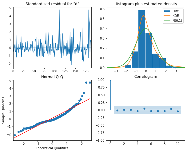
Finally, we will forecast and evaluate the results against our previously used baseline of the last known forecast. We will also compare the ARMA(0, 2) forecast with results from our previous AR(4) and MA(2) forecasts.
As we can see by the function call, an ARMA(0, 2) is equivalent to an MA(2) process. We expect the results from these models to be the same.
PYTHON
TRAIN_LEN = len(train)
HORIZON = len(test)
WINDOW = 1

pred_last_value = last_known(df_diff, TRAIN_LEN, HORIZON, WINDOW)
pred_MA = model_forecast(df_diff, TRAIN_LEN, HORIZON, 0, 2, WINDOW)
pred_AR = model_forecast(df_diff, TRAIN_LEN, HORIZON, 4, 0, WINDOW)
pred_ARMA = model_forecast(df_diff, TRAIN_LEN, HORIZON, 0, 2, WINDOW)

test['pred_last_value'] = pred_last_value
test['pred_MA'] = pred_MA
test['pred_AR'] = pred_AR
test['pred_ARMA'] = pred_ARMA

print(test.head())
OUTPUT
     daily_usage  pred_last_value   pred_MA   pred_AR  pred_ARMA
189     -13.5792          -1.8630 -1.870535  1.735114  -1.870535
190     -10.8660         -13.5792  4.425102  5.553305   4.425102
191       4.8054         -10.8660  9.760944  9.475778   9.760944
192       6.2280           4.8054  7.080340  5.395541   7.080340
193      -5.6718           6.2280  2.106354  0.205880   2.106354
Indeed, we can see the results for the “pred_MA” and “pred_ARMA” forecasts are the same. While that may seem underwhelming, it’s important to note that in this case our model was determined using a statistical approach to fitting multiple models, whereas previously we manually counted significant lags in an ACF plot. This approach is much more scalable.
Since the results are the same, we will only refer to the “pred_ARMA” results from here on when comparing against the baseline and the “pred_AR” results.
The plot indicates that the forecasts of the AR(4) model and the ARMA(0,2) model are very similar.
PYTHON
fig, ax = plt.subplots()

ax.plot(df_diff[150:]['daily_usage'], 'b-', label='actual')
ax.plot(test['pred_last_value'], 'r-.', label='last')
ax.plot(test['pred_AR'], 'g--', label='AR(4)')
ax.plot(test['pred_ARMA'], 'k--', label='ARMA(0,2)')

ax.axvspan(189, 211, color='#808080', alpha=0.2)
ax.legend(loc=2)

ax.set_xlabel('Time')
ax.set_ylabel('Energy use - diff')

plt.tight_layout()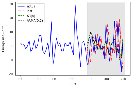
The mean squared error shows a meaningful improvement from the results of the AR(4) model in the previous section.
PYTHON
mse_last = mean_squared_error(test['daily_usage'], test['pred_last_value'])
mse_AR = mean_squared_error(test['daily_usage'], test['pred_AR'])
mse_ARMA = mean_squared_error(test['daily_usage'], test['pred_ARMA'])

print("MSE of last known value forecast:", mse_last)
print("MSE of AR(4) forecast:",mse_AR)
print("MSE of ARMA(0, 2) forecast:",mse_ARMA)
OUTPUT
MSE of last known value forecast: 252.6110739163637
MSE of AR(4) forecast: 85.29189129936279
MSE of ARMA(0, 2) forecast: 73.404918547051
We perform the reverse transformation on the forecasts from the differenced data to apply them to the source data.
PYTHON
daily_usage['pred_usage'] = pd.Series()
daily_usage['pred_usage'][190:] = daily_usage['sum'].iloc[190] + test['pred_ARMA'].cumsum()
print(daily_usage.tail())
OUTPUT
                   sum  pred_usage
INTERVAL_TIME
2019-07-27     23.2752   39.668821
2019-07-28     42.0504   37.635355
2019-07-29     36.6444   27.803183
2019-07-30     18.0828   19.441330
2019-07-31     25.5774   23.182106
We evaluate the transformed forecasts using the mean absolute error.
PYTHON
mae_MA_undiff = mean_absolute_error(daily_usage['sum'].iloc[190:],
                                    daily_usage['pred_usage'].iloc[190:])

print("Mean absolute error, ARMA(0, 2):", mae_MA_undiff)
OUTPUT
Mean absolute error, ARMA(0, 2): 15.766473755136264Finally, we can visualize the forecasts in comparison with the actual values.
PYTHON
fig, ax = plt.subplots()

ax.plot(daily_usage['sum'].values, 'b-', label='actual')
ax.plot(daily_usage['pred_usage'].values, 'k--', label='ARMA(0,2)')

ax.legend(loc=2)

ax.set_xlabel('Time')
ax.set_ylabel('Energy consumption')
ax.axvspan(161, 180, color='#808080', alpha=0.2)

fig.autofmt_xdate()
plt.tight_layout()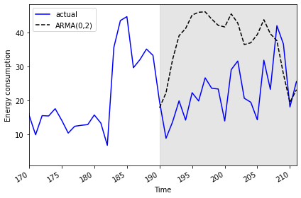
Key Points
- The Akaike information criterion (AIC) is an attribute of a SARIMAX model that can be used to compare model results using different ARMA(p, q) parameters.